Z-Score in Statistics

Z-Score in statistics measures how many standard deviations a data point lies away from the mean of a distribution. It standardizes values across different distributions, enabling meaningful comparisons even when datasets have different means and standard deviations. It is widely used in hypothesis testing, outlier detection and normalizing data for machine learning models.

• Z-score of 0 means the data point is exactly at the mean.
• Positive Z-score indicates the data point is above the mean.
• Negative Z-score indicates the data point is below the mean.
• To calculate a Z-score, the population mean (\mu) and population standard deviation (\sigma) must be known.

For example, a Z-score of 2 means the value is 2 standard deviations above the mean, placing it in the top \sim 2.3\% of a normal distribution.

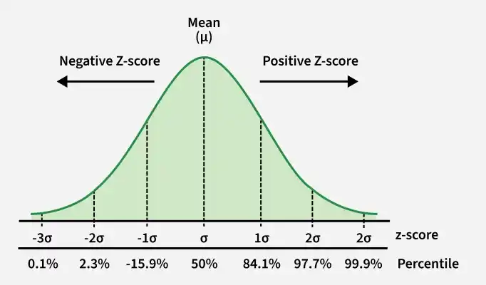
Z-score is a statistical measure that describes a value's position relative to the mean, expressed in terms of standard deviations, indicating how far and in which direction a data point deviates from the mean.

Z-Score Formula

To calculate the Z-score of a data point, we need the value of the element, the population mean and the population standard deviation:

z = \frac{X - \mu}{\sigma}

Where:

• z: Z-Score
• X: Value of the data point
• \mu: Population Mean
• \sigma: Population Standard Deviation

Properties of Z-Score

1. Allows comparison of data points from different distributions by standardizing values on a common scale.

2. |Z| > 2 is considered unusual or statistically significant, while |Z| > 3 is typically flagged as an outlier, extremely far from the mean.

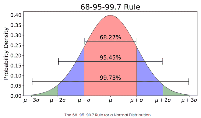
3. Z-scores follow the Empirical Rule in a normal distribution:

• 68% of data points have a Z-score between -1 and 1.
• 95% of data points have a Z-score between -2 and 2.
• 99% of data points have a Z-score between -3 and 3.

How to Calculate Z-Score

To calculate the Z-score, substitute the observed value (X), population mean (\mu), and population standard deviation (\sigma) into the Z-score formula. Depending on whether the result is positive or negative, use the corresponding positive Z-Table or negative Z-Table to find the cumulative probability.

Example 1: You score 500 on the GATE examination. The mean score is 390 and the standard deviation is 45. How well did you perform compared to other test-takers?

Soluction:

Given: X = 500, \mu = 390, \sigma = 45

z = \frac{X-\mu}{\sigma}= \frac{500-390}{45}= \frac{110}{45}\approx 2.44

Since the Z-score is positive, use the positive Z-Table:

1. Map 2.4 on the Y-axis.
2. Map 0.04 on the X-axis.
3. The intersection gives a cumulative probability of 0.99266.

This probability represents the area under the standard normal curve to the left of the Z-score

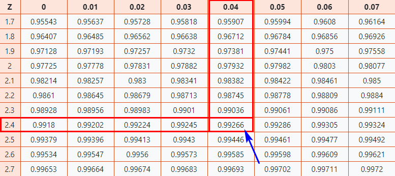
From the Z-Table, the cumulative probability for Z = 2.44 is 0.99266. Converting to percentage:

0.99266 \times 100 = 99.266\%

This means you performed better than approximately 99% of other test-takers.

Example 2: What is the probability that a student scores between 350 and 400 (with a mean score \mu of 390 and a standard deviation \sigma of 45)?

Solution:

Given : X_1 = 350,\quad X_2 = 400,\quad \mu = 390,\quad \sigma = 45

z_1 = \frac{350 - 390}{45} = \frac{-40}{45} \approx -0.89

Since z_{1} is negative, use the negative Z-Table: p_{1}=0.18943

z_2 = \frac{400 - 390}{45}= \frac{10}{45}\approx 0.22

Since z_{2}​ is positive, use the positive Z-Table: p_{2}=0.58706

The final probability is computed by subtracting p_{1} from p_{2}

p = p_2 - p_1= 0.58706 - 0.18943= 0.39763

The probability that a student scores between 350 and 400 is 39.763%.

Calculating Outliers Using Z-Score

Z-scores can be used to detect outliers by identifying data points that lie too far from the mean. A common cutoff threshold is |Z| > 3, meaning the data point falls outside 99.73% of the distribution.

• Calculate the mean (μ) and standard deviation (σ) of the dataset, then compute the Z-score for each data point.
• Define a cutoff threshold (commonly 2 or 3) based on project requirements.
• Any data point exceeding the cutoff is classified as an outlier and can be removed or treated accordingly.

Refer Z score for Outlier Detection - Python

Example 1: A dataset has a mean (\mu) of 70 and standard deviation (\sigma) of 5. Determine whether the data point X = 80 is an outlier.

Solution:

Given: X = 80,\quad \mu = 70,\quad \sigma = 5

z = \frac{X - \mu}{\sigma}= \frac{80 - 70}{5}= \frac{10}{5}= 2

Since |Z| = 2 < 3, the data point is not an outlier, but it is 2 standard deviations above the mean, which may be considered unusual depending on the chosen threshold.

Example 2: A dataset of exam scores: 75, 82, 90, 68, 95. Determine whether the score 82 is an outlier.

Solution:

Step 1: Calculate the mean

\mu = \frac{75 + 82 + 90 + 68 + 95}{5}= \frac{410}{5}= 82

Step 2: Calculate the standard deviation

\sigma = \sqrt{\frac{(-7)^2 + 0^2 + 8^2 + (-14)^2 + 13^2}{4}} = \sqrt{\frac{466}{4}} \approx 10.79

Step 3: Calculate the Z-Score for 82

z = \frac{82 - 82}{10.79}= \frac{0}{10.79}= 0

Since |Z| = 0, the score of 82 lies exactly at the mean and is clearly not an outlier.

Implementation

We calculate Z-scores and detect outliers in a dataset. The NumPy library is used to efficiently compute the mean and standard deviation across the dataset.

• Compute the mean and standard deviation of the dataset using np.mean() and np.std().
• Calculate the Z-score for each data point by subtracting the mean and dividing by the standard deviation.
• Flag any data point with a Z-score greater than 3 as an outlier, as it lies outside 99.73% of the distribution.

import numpy as np

def calculate_z_score(data):
  # Mean of the dataset 
    mean = np.mean(data)
   # Standard Deviation of tha dataset 
    std_dev = np.std(data)
   # Z-score of tha data points 
    z_scores = (data - mean) / std_dev
    return z_scores

# Example dataset 
dataset = [3,9, 23, 43,53, 4, 5,30, 35, 50, 70, 150, 6, 7, 8, 9, 10]
z_scores = calculate_z_score(dataset)
print('Z-Score :',z_scores)

# Data points which lies outside 3 standard deviatioms are outliers 
# i.e outside range of99.73% values
outliers = [data_point for data_point, \
          z_score in zip(dataset, z_scores) if z_score > 3]
print(f'\nThe outliers in the dataset is {outliers}')

Output:

Z-Score : [-0.7574907 -0.59097335 -0.20243286 0.35262498 0.6301539 -0.72973781
-0.70198492 -0.00816262 0.13060185 0.54689523 1.10195307 3.32218443
-0.67423202 -0.64647913 -0.61872624 -0.59097335 -0.56322046]
The outliers in the dataset is [150]

Applications

• Feature Scaling: Standardizes features to a common scale, helping algorithms like KNN and SVM treat all features equally.
• Outlier Detection: Identifies outliers by flagging data points with Z-scores beyond \pm3, indicating they are far from the average.
• Anomaly Detection: Detects rare or unexpected events in data that deviate significantly from normal behavior, useful in fraud detection and quality control.
• Regression Diagnostics: Checks residuals in regression models — Z-scores far from 0 may indicate issues like heteroscedasticity or poor model fit.
• Comparing Different Distributions: Enables fair comparison of values from datasets with different units, means or scales such as comparing test scores across different exams.

Z-Scores vs. Standard Deviation

Related Articles

• Z-Score in Statistics
• Z-Score Table