A Threaded PyQt GUI and Particles

I wrote a post about adding a GUI to your command line interface program. Sometimes people just want to click stuff. If you tried it / implemented it yourself, you'd have seen that the program would have gone from responsive to non-responsive when you hit the run button. Why? Because the program can only do ONE think at a time and frankly, keeping the controls available for clicking at all times, updating the graphics and calculating particle movement do not get along nicely. This post is about making it behave like we expect.

I present to you threading. Specifically for PyQt there is the QThread class which is actually discussed rather nicely in this PyQtWiki and this page by Jo Plaete which I used for inspiration.

What complicates the whole scene is that we need to realize that we have two independant things we want to accomplish: 1) move particles and 2) update the graphics. Both independent of the GUI.

I started by making my own class called BaseThread which subclasses QThread. The code is

where I believe the magic for everything not just crashing and burning is the subtle use of the custom boolean flag exiting (which we will use later) and the use of self.wait() in the __del__ method. Again, for details you should read the blog posts mentioned above.

To come around many of the syncronization problems that arises with threads the Qt framework allows us to use custom signals to make everything talk together. Here is my version of a StepThread which defines the run method (you do NEVER call this explicitly!) and a convenience function called simulate to start a simulation for N steps. The run function emits a custom signal and sleeps for a little while before simulating again.

Very similarly we have the DrawThread which emits a signal so we can update the matplotlib surface.

Notice that it updates less frequently. I have yet to figure out something clever in this regard.

Finally, I had to make some tweaks to the Simulator class (nothing very fancy) to hook up our custom signals.

What I need now is a video of it and maybe to implement some different potentials instead of only the non-interacting particles. Stay tuned.

The entire code can be downloaded from the latest gist I made.

Obtaining Contact Numbers using SMARTS

Because I'm on a roll with blogging right now and I am looking for excuses to not write the next paper, here is a post about how to utilize SMARTS[1] for something cheminformatically-vant such as the contact number[2]. We will base the new code on what I did in the last post I wrote. The contact number is basically "Select an $\alpha$-Carbon and count the number $\alpha$-Carbons within a sphere of a certain radius $R$ from it". This give rise to a 1D measurement (see below) of how buried residues are. If you massage your data enough (we will get to this in a later post) it can be used to validate whether a protein is folded (somewhat) correctly or not. There is much more to this story than I have room for on my blog, but I do recommend you follow the blog of Anders Christensen, a fellow student who folds more proteins than I.

Our work today shall start from Crambine (PDB: 1CRN) which I've prepared for your viewing pleasure in pymol

From last week, the boiler-plate code we shall start from is

import openbabel
filename = "1CRN.pdb"
pattern = "[$(CC(=O)[N,O])]"
obmol = openbabel.OBMol()
obpat = openbabel.OBSmartsPattern()
obconv = openbabel.OBConversion()
obconv.SetInFormat(filename[-3:])
obconv.ReadFile(obmol, filename)
obpat.Init(pattern)
obpat.Match(obmol)
alpha_carbons = [m[0] for m in obpat.GetUMapList()]

I'm interested in $\alpha$-Carbons so the atomic primitive pattern we use to match with will be

[$(CC(=O)[N,O])]

The last part, [N,O] is a match of either a Nitrogen or an Oxygen. This Oxygen match is needed for the C-terminal. Because we are using SMARTS, this is the only thing that will change in our code once it is done. Should we be interested in locating the carboxyl groups of the backbone for instance, simply change one pattern. Of course, if you want to match $\alpha$-Carbons to carboxyl groups, this requires an extra pattern match.

Running this code will return a list of atoms. To calculate the contact number, the following function iterates over each match, forms a pair with all other matches and calculates the contact number for one residue at a time

def ContactNumbersForCutoff(matches, rcut):
  contact_numbers = []
  for i in matches:
    contact_number = 0 
    ai = obmol.GetAtom(i)
    for j in matches:
      if i == j: continue
      aj = obmol.GetAtom(j)
      if ai.GetDistance(aj) < rcut:
        contact_number +=1

    contact_numbers.append(contact_number)
  return contact_numbers

which we will invoke to generate the list of contact numbers

cn12 = ContactNumbersForCutoff(alpha_carbons, 12.0)

Since I am fond of the matplotlib[3] library for python when dealing with plots and I don't feel like doing the hard work myself anyways, I'll just plot[4] the list of numbers using the following code

pylab.plot(cn12)
pylab.savefig("contact.png")

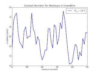
which (after some additional touches - see the github page for the final code) results in

Here we see that residues 20, 38, 39 and 40 are clearly not buried when compared to residues 30 to 36. In a later posts, I will add a few lines of code to calculate the above information in a slightly more useful way. I'd also like to explore a quick implementation of the Half-Sphere Exposure[5] method instead as it provides even more clue to the local environment.

check out the source code on my github page.