🔥 ข่าวด่วน: ed/Sampling Algorithms/The Rejection Method.html

A.3 The Rejection Method

Many functions cannot be integrated in order to normalize them to find their PDFs. Even given a PDF, it is often not possible to invert the associated CDF to generate samples using the inversion method. In such cases, the rejection method can be useful: it is a technique for generating samples according to a function’s distribution without needing to do either of these steps. Assume that we want to draw samples from some function where we have some PDF that satisfies for a constant , and suppose that we do know how to sample from . The rejection method is then:

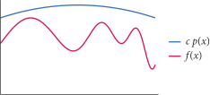
This procedure repeatedly chooses a pair of random variables . If the point lies under , then the sample is accepted. Otherwise, it is rejected and a new sample pair is chosen. This idea is illustrated in Figure A.2; it works in any number of dimensions. It should be evident that the efficiency of this scheme depends on how tightly bounds .

Figure A.2: Rejection sampling generates samples according to the distribution of a function even if ’s PDF is unknown or its CDF cannot be inverted. If some distribution and a scalar constant are known such that , then samples can be drawn from and randomly accepted in a way that causes the accepted samples to be from ’s distribution. The closer the fit of to , the more efficient this process is.

For example, suppose we want to select a uniformly distributed point inside a unit disk. Using the rejection method, we simply select a random position inside the circumscribed square and return it if it falls inside the disk. This process is shown in Figure A.3.

Figure A.3: Rejection Sampling a Disk. One approach to finding uniform points in the unit disk is to sample uniform random points in the unit square and reject all that lie outside the disk (red points). The remaining points will be uniformly distributed within the disk.

The function RejectionSampleDisk() implements this algorithm. A similar approach will work to generate uniformly distributed samples on the inside of any complex shape as long as it has an inside–outside test.

<<Sampling Function Definitions>>+=

Point2f RejectionSampleDisk(RNG &rng) { Point2f p; do { p.x = 1 - 2 * rng.Uniform<Float>(); p.y = 1 - 2 * rng.Uniform<Float>(); } while (Sqr(p.x) + Sqr(p.y) > 1); return p; }

In general, the efficiency of rejection sampling depends on the percentage of samples that are expected to be rejected. For RejectionSampleDisk(), this is easy to compute. It is the area of the disk divided by the area of the square: . If the method is applied to generate samples in hyperspheres in the general -dimensional case, however, the volume of an -dimensional hypersphere goes to 0 as increases, and this approach becomes increasingly inefficient.

Rejection sampling is not used in any of the Monte Carlo algorithms currently implemented in pbrt. We will normally prefer to find distributions that are similar to the function that can be sampled directly, so that well-distributed sample points in can be mapped to sample points that are in turn well distributed. Nevertheless, rejection sampling is an important technique to be aware of, particularly when debugging Monte Carlo implementations. For example, if one suspects the presence of a bug in code that draws samples from some distribution using the inversion method, then one can replace it with a straightforward implementation based on the rejection method and see if the Monte Carlo estimator converges to the same value. Of course, it is necessary to take many samples in situations like these, so that variance in the estimates does not mask errors.