Discrete Fourier Transform and its Inverse using MATLAB

The Discrete Fourier Transform (DFT) and Inverse Discrete Fourier Transform (IDFT) are fundamental techniques in Digital Signal Processing (DSP). The DFT converts a discrete-time signal from the time (or spatial) domain into the frequency domain, making it possible to analyze the frequency components present in the signal.

• The IDFT performs the reverse operation by reconstructing the original signal from its frequency-domain representation.
• MATLAB provides built-in functions as well as matrix-based implementations for understanding and visualizing these transforms.

Mathematical Foundations

The DFT and IDFT are mathematically defined using the following equations.

DFT: The Discrete Fourier Transform (DFT) of a sequence x(n) of length N is:

X(k) = \sum_{n=0}^{N-1} x(n) \cdot e^{-j 2\pi k n / N}

Where:

• x(n) is the input time-domain sequence.
• X(k) is the frequency-domain representation.
• N is the total number of samples.
• n=0, 1,…,N−1
• k=0,1,…,N−1

IDFT: The Inverse Discrete Fourier Transform (IDFT) reconstructs the original sequence:

x(n) = \frac{1}{N} \sum_{k=0}^{N-1} X(k) \cdot e^{j 2\pi k n / N}

Where:

• X(k) is the frequency-domain sequence.
• x(n)is the reconstructed time-domain signal.
• N is the total number of samples.
• n=0,1,…,N−1
• k=0,1,…,N−1

Matrix Representation

The DFT and IDFT can also be represented as matrix multiplications. The exponential terms (commonly called twiddle factors) form an N×N transformation matrix. Multiplying this matrix by the input vector computes the DFT, while multiplying by the corresponding inverse transformation matrix and dividing by N reconstructs the original signal.

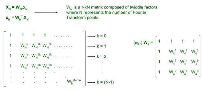
If the input signal is represented as an N×1 column vector, the output obtained after matrix multiplication is also an N×1 column vector.

DFT in MATLAB

1. Define the input sequence and the required number of DFT points NNN.
2. Zero-pad the sequence if its length is smaller than NNN.
3. Construct the DFT transformation matrix using the exponential twiddle factors.
4. Multiply the transformation matrix by the input vector to obtain the DFT coefficients.
5. Plot the magnitude and phase spectra.

clc;
xn=input('Input sequence: ');
N = input('Enter the number of points: ');
Xk=calcdft(xn,N);
disp('DFT X(k): ');
disp(Xk);
mgXk = abs(Xk);
phaseXk = angle(Xk);
k=0:N-1;
subplot (2,1,1);
stem(k,mgXk);
title ('DFT sequence: ');
xlabel('Frequency');
ylabel('Magnitude');
subplot(2,1,2);
stem(k,phaseXk);
title('Phase of the DFT sequence');
xlabel('Frequency');
ylabel('Phase');

function[Xk] = calcdft(xn,N)
    L=length(xn);
    if(N<L)
        error('N must be greater than or equal to L!!')
    end
    x1=[xn, zeros(1,N-L)];
    for k=0:1:N-1
        for n=0:1:N-1
            p=exp(-i*2*pi*n*k/N);
            W(k+1,n+1)=p;
        end
    end
    disp('Transformation matrix for DFT')
    disp(W);
    Xk=W*(x1.')
end

Output:

>> Input sequence: [1 4 9 16 25 36 49 64 81]
>> Enter the number of points: 9

• The input sequence is zero-padded if needed to match N.
• The DFT matrix W is explicitly built using nested loops.
• The output Xk contains complex-valued frequency-domain samples.
• The code displays both the magnitude and phase spectrum with stem plots which are standard for discrete data.

IDFT in MATLAB

1. Provide the frequency-domain sequence X(k)X(k)X(k).
2. Construct the IDFT transformation matrix using positive exponential terms.
3. Multiply the transformation matrix by the frequency-domain vector.
4. Divide the result by NNN to reconstruct the original time-domain signal.
5. Plot the reconstructed signal.

clc;
Xk = input('Input sequence X(k): ');
xn=calcidft(Xk);
N=length(xn);
disp('xn');
disp(xn);
n=0:N-1;
stem(n,xn);
xlabel('time');
ylabel('Amplitude');

function [xn] = calcidft(Xk)
    N=length(Xk);
    for k=0:1:N-1
        for n=0:1:N-1
            p=exp(i*2*pi*n*k/N);
            IT(k+1,n+1)=p;
        end
    end
    disp('Transformation Matrix for IDFT');
    disp(IT);
    xn = (IT*(Xk.'))/N;
end

Output:

>> Enter the input sequence: [1 2 3 4 5 9 8 7 6 5]

• The IDFT matrix is constructed similarly but uses exp (+1i*...) to inverse the frequency components.
• The output is divided by N, as required by the mathematical formula.
• Output is plotted using stem for a clear, discrete view.