Latent Class Analysis in R

Latent Class Analysis (LCA) is a statistical method used to identify unobserved subgroups (latent classes) within a population based on individuals' responses to observed categorical variables. It is widely applied in psychology, sociology, marketing, epidemiology and education to uncover hidden structures and patterns within data.

• Models the probability of membership in latent classes to understand population heterogeneity.
• Helps simplify complex data structures by grouping individuals with similar response patterns into distinct subgroups.
• Assumes that observed associations between variables are explained by membership in an underlying latent class.
• Useful for market segmentation, patient profiling, behavioral research and educational assessment.

In R Language, packages such as poLCA, flexmix, and Mclust provide robust functions for conducting LCA.

Implementing Latent Class Analysis in R

The poLCA package in R performs LCA using a finite mixture modeling approach. Below is a step-by-step guide to conduct LCA using poLCA.

Step 1: Installing and Load the required Packages

Now we will install and load the required Packages.

# Install and load the poLCA package
install.packages("poLCA")
library(poLCA)

Step 2: Data Preparation

LCA requires categorical variables as input, where responses must be coded as positive integers starting from 1 (e.g., 1, 2, 3). These integer codes are treated as categorical/nominal labels, not numerical quantities.

• Non-Likert scale survey responses can also be coded as 1, 2, 3... as long as each integer represents a distinct category.
• The numeric value itself has no mathematical meaning it is simply a label for a response category.

# Simulated dataset
set.seed(123)
survey_data <- data.frame(
  Q1 = sample(1:3, 1000, replace = TRUE),
  Q2 = sample(1:4, 1000, replace = TRUE),
  Q3 = sample(1:3, 1000, replace = TRUE),
  Q4 = sample(1:4, 1000, replace = TRUE),
  Q5 = sample(1:3, 1000, replace = TRUE)
)
head(survey_data)

Output:

  Q1 Q2 Q3 Q4 Q5
1  3  4  1  4  3
2  3  2  3  1  2
3  3  3  3  1  2
4  2  2  2  4  1
5  3  4  1  2  3
6  2  4  3  2  1

This creates a simulated dataset with 1,000 respondents answering 5 questions (Q1 to Q5), with responses sampled randomly from specified category ranges.

Step 3: Model Specification

To specify an LCA model, use the poLCA function from the poLCA package. Define a formula indicating the observed variables and set the number of latent classes we want to extract.

# Specifying the LCA model with 3 latent classes
f <- cbind(Q1, Q2, Q3, Q4, Q5) ~ 1
lca_model <- poLCA(f, survey_data, nclass = 3)

Output:

Conditional item response (column) probabilities,
by outcome variable, for each class (row)

$Q1
Pr(1) Pr(2) Pr(3)
class 1: 0.2480 0.4188 0.3332
class 2: 0.3746 0.3205 0.3050
class 3: 0.3310 0.2679 0.4011

$Q2
Pr(1) Pr(2) Pr(3) Pr(4)
class 1: 0.1712 0.0517 0.5381 0.2390
class 2: 0.2215 0.2758 0.2750 0.2278
class 3: 0.3626 0.3964 0.0000 0.2409

$Q3
Pr(1) Pr(2) Pr(3)
class 1: 0.3559 0.2420 0.4020
class 2: 0.2997 0.2923 0.4079
class 3: 0.3595 0.3989 0.2416

$Q4
Pr(1) Pr(2) Pr(3) Pr(4)
class 1: 0.2073 0.5334 0.0097 0.2497
class 2: 0.2022 0.0474 0.5650 0.1853
class 3: 0.3243 0.3391 0.0019 0.3346

$Q5
Pr(1) Pr(2) Pr(3)
class 1: 0.2819 0.3847 0.3334
class 2: 0.3308 0.3066 0.3625
class 3: 0.3138 0.4112 0.2750

Estimated class population shares
0.2754 0.4101 0.3144

Predicted class memberships (by modal posterior prob.)
0.245 0.311 0.444

=========================================================
Fit for 3 latent classes:
=========================================================
number of observations: 1000
number of estimated parameters: 38
residual degrees of freedom: 393
maximum log-likelihood: -6044.248

AIC(3): 12164.5
BIC(3): 12350.99
G^2(3): 462.2892 (Likelihood ratio/deviance statistic)
X^2(3): 397.0556 (Chi-square goodness of fit)

ALERT: iterations finished, MAXIMUM LIKELIHOOD NOT FOUND

The output is organized into four key components:

1. Conditional Item Response Probabilities

These represent the probability of observing each response category for each question within each latent class.

• $Q1 to $Q5: Each section corresponds to one survey question.
• Pr(1) to Pr(4): Each column represents a response category. For example, Pr(1) is the probability of selecting category 1, Pr(2) for category 2 and so on.
• class 1 to class 3: Each row represents a latent class. The probabilities within each row indicate how likely individuals in that class are to choose each response option for that question.

2. Estimated Class Population Shares vs. Predicted Class Memberships

These are two distinct concepts:

• Estimated Class Population Shares (0.2754, 0.4101, 0.3144): Model-level estimates of the proportion of the overall population belonging to each latent class, derived probabilistically from model parameters.
• Predicted Class Memberships (0.245, 0.311, 0.444): Proportion of individuals hard-assigned to each class based on their highest posterior probability. Differs from population shares when class membership is uncertain or mixed.

3. Fit Statistics

These assess how well the model fits the observed data:

• AIC (Akaike Information Criterion): Measures relative model quality, lower values indicate better fit.
• BIC (Bayesian Information Criterion): Similar to AIC but penalizes model complexity more heavily; preferred for model selection with lower values indicating better fit.
• G² (Likelihood Ratio/Deviance Statistic): Goodness-of-fit based on the difference between observed and expected frequencies, smaller values indicate better fit.
• X² (Chi-square Goodness of Fit): Goodness-of-fit based on the chi-square distribution, smaller values indicate better fit.
• Maximum Log-Likelihood (-6044.248): The maximum value of the log-likelihood function achieved during estimation.

4. Convergence Alert

The "ALERT: iterations finished, MAXIMUM LIKELIHOOD NOT FOUND" warning indicates that the EM algorithm converged but failed to find the true maximum likelihood, suggesting potential convergence issues.

• Increase nrep to run more random starts and improve the chances of finding the global maximum.
• Try different random seeds using set.seed() to explore different starting points.

Overall, the relatively low AIC and BIC values suggest the 3-class model adequately describes the observed data, but the convergence alert should be addressed before drawing final conclusions.

Step 4: Estimation Methods

poLCA uses the Expectation-Maximization (EM) algorithm to estimate model parameters by iteratively maximizing the likelihood of the observed data. Multiple random starts (nrep) are used to avoid local maxima.

# Fitting the model with multiple random starts
lca_model <- poLCA(f, survey_data, nclass = 3, nrep = 5)

Output:

Model 1: llik = -6044.317 ... best llik = -6044.317
Model 2: llik = -6044.172 ... best llik = -6044.172
Model 3: llik = -6044.023 ... best llik = -6044.023
Model 4: llik = -6044.239 ... best llik = -6044.023
Model 5: llik = -6044.085 ... best llik = -6044.023
Conditional item response (column) probabilities,
by outcome variable, for each class (row)

$Q1
Pr(1) Pr(2) Pr(3)
class 1: 0.3065 0.2906 0.4029
class 2: 0.3746 0.3145 0.3109
class 3: 0.1756 0.4752 0.3492

$Q2
Pr(1) Pr(2) Pr(3) Pr(4)
class 1: 0.3899 0.3527 0.0000 0.2574
class 2: 0.2220 0.2655 0.2852 0.2273
class 3: 0.0956 0.0000 0.6838 0.2206

$Q3
Pr(1) Pr(2) Pr(3)
class 1: 0.3722 0.3875 0.2403
class 2: 0.2979 0.2966 0.4055
class 3: 0.3987 0.2225 0.3789

$Q4
Pr(1) Pr(2) Pr(3) Pr(4)
class 1: 0.3081 0.3336 0.0001 0.3582
class 2: 0.2337 0.1577 0.4150 0.1937
class 3: 0.1436 0.6016 0.0001 0.2547

$Q5
Pr(1) Pr(2) Pr(3)
class 1: 0.3110 0.4326 0.2564
class 2: 0.3331 0.3126 0.3543
class 3: 0.2318 0.4076 0.3606

Estimated class population shares
0.2883 0.5662 0.1456

Predicted class memberships (by modal posterior prob.)
0.363 0.518 0.119

=========================================================
Fit for 3 latent classes:
=========================================================
number of observations: 1000
number of estimated parameters: 38
residual degrees of freedom: 393
maximum log-likelihood: -6044.023

AIC(3): 12164.05
BIC(3): 12350.54
G^2(3): 461.8389 (Likelihood ratio/deviance statistic)
X^2(3): 397.9841 (Chi-square goodness of fit)

ALERT: iterations finished, MAXIMUM LIKELIHOOD NOT FOUND

It suggest that the model with 3 latent classes adequately describes the observed data, as indicated by relatively low AIC and BIC values and reasonable goodness-of-fit statistics. However, the alert regarding the maximum likelihood not being found warrants further investigation into the convergence of the estimation process.

Step 5: Model Selection

Choosing the optimal number of latent classes is crucial. Fit multiple models with different numbers of classes and compare their fit using criteria such as the Bayesian Information Criterion (BIC) and Akaike Information Criterion (AIC).

bic_values <- numeric()
aic_values <- numeric()

for (k in 1:5) {
  lca_model_k <- poLCA(f, survey_data, nclass = k, nrep = 5)
  bic_values[k] <- lca_model_k$bic
  aic_values[k] <- lca_model_k$aic
}

Output:

Conditional item response (column) probabilities,
by outcome variable, for each class (row)

$Q1
Pr(1) Pr(2) Pr(3)
class 1: 0.3065 0.2906 0.4029
class 2: 0.3746 0.3145 0.3109
class 3: 0.1756 0.4752 0.3492

$Q2
Pr(1) Pr(2) Pr(3) Pr(4)
class 1: 0.3899 0.3527 0.0000 0.2574
class 2: 0.2220 0.2655 0.2852 0.2273
class 3: 0.0956 0.0000 0.6838 0.2206

$Q3
Pr(1) Pr(2) Pr(3)
class 1: 0.3722 0.3875 0.2403
class 2: 0.2979 0.2966 0.4055
class 3: 0.3987 0.2225 0.3789

$Q4
Pr(1) Pr(2) Pr(3) Pr(4)
class 1: 0.3081 0.3336 0.0001 0.3582
class 2: 0.2337 0.1577 0.4150 0.1937
class 3: 0.1436 0.6016 0.0001 0.2547

$Q5
Pr(1) Pr(2) Pr(3)
class 1: 0.3110 0.4326 0.2564
class 2: 0.3331 0.3126 0.3543
class 3: 0.2318 0.4076 0.3606

Estimated class population shares
0.2883 0.5662 0.1456

Predicted class memberships (by modal posterior prob.)
0.363 0.518 0.119

=========================================================
Fit for 3 latent classes:
=========================================================
number of observations: 1000
number of estimated parameters: 38
residual degrees of freedom: 393
maximum log-likelihood: -6044.023

AIC(3): 12164.05
BIC(3): 12350.54
G^2(3): 461.8389 (Likelihood ratio/deviance statistic)
X^2(3): 397.9841 (Chi-square goodness of fit)

ALERT: iterations finished, MAXIMUM LIKELIHOOD NOT FOUND

The results show the response probabilities for each question within each latent class, the estimated size of each class, and the predicted class memberships. The model fit indices suggest that the model is reasonably fitting the data, although the alert about the maximum likelihood not being found indicates a potential issue that might require further attention.

Step 6: Visualization

Visualizing the results of LCA can enhance understanding and communication of the findings. Plotting the item-response probabilities for each class helps in interpreting the distinct profiles of the latent classes.

# Class membership probabilities
lca_model$P

# Item-response probabilities
lca_model$probs
# Example visualization of item-response probabilities
plot_lca <- function(lca_model) {
  probs <- lca_model$probs
  num_classes <- length(probs)
  par(mfrow = c(1, num_classes))
  
  for (i in 1:num_classes) {
    barplot(t(as.matrix(probs[[i]])), beside = TRUE, col = rainbow(ncol(probs[[i]])),
            main = paste("Class", i), xlab = "Questions", ylab = "Probability")
  }
}

plot_lca(lca_model)

Output:

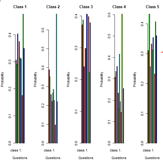
The visualization of item-response probabilities provides a comprehensive overview of the response patterns within each latent class, allowing for deeper insights into the underlying structure of the data analyzed using latent class analysis.

Download full code from here.