Mahotas - Parameter-Free Threshold Adjacency Statistics

In this article we will see how we can get the image's parameter-free threshold adjacency statistics in mahotas. TAS were presented by Hamilton et al. in “Fast automated cell phenotype image classification” 
For this tutorial we will use 'lena' image, below is the command to load the lena image 

mahotas.demos.load('lena')

Below is the lena image  

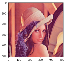
In order to do this we will use mahotas.features.pftas method
Syntax : mahotas.features.pftas(img)
Argument : It takes image object as argument
Return : It returns 1-D array 
 

Note : Input image should be filtered or should be loaded as grey

In order to filter the image we will take the image object which is numpy.ndarray and filter it with the help of indexing, below is the command to do this

image = image[:, :, 0]

Below is the implementation 

# importing required libraries
import mahotas
import mahotas.demos
from pylab import gray, imshow, show
import numpy as np
import matplotlib.pyplot as plt
  
# loading image
img = mahotas.demos.load('lena')
  
# filtering image
img = img.max(2)

print("Image")
  
# showing image
imshow(img)
show()

# computing pftas
value = mahotas.features.pftas(img)
 

# printing value
print(value)

Output :

Image 

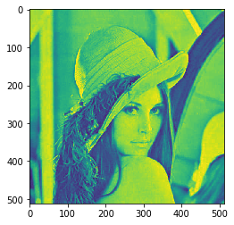
[8.40466496e-01 3.96107929e-02 3.32482230e-02 4.78710924e-02
 1.99986198e-02 9.29542475e-03 4.81678283e-03 3.41591333e-03
 1.27665448e-03 8.74954977e-01 3.30841335e-02 2.54587942e-02
 3.93565900e-02 1.67089809e-02 5.66629477e-03 2.56520631e-03
 1.63400128e-03 5.71021954e-04 8.94910256e-01 2.94171187e-02
 2.18929382e-02 3.09704979e-02 1.29246004e-02 5.15770440e-03
 2.69414206e-03 1.49270033e-03 5.40041990e-04 7.95067984e-01
 5.76368630e-02 4.24876742e-02 5.77221625e-02 2.45406623e-02
 1.12339424e-02 7.21633656e-03 3.25844038e-03 8.35934968e-04
 9.01310067e-01 2.80622737e-02 1.99915045e-02 3.05637402e-02
 1.27837749e-02 4.03875587e-03 1.90138423e-03 1.03160208e-03
 3.16897372e-04 8.28594029e-01 4.43179717e-02 3.44044708e-02
 5.11290091e-02 2.25801812e-02 1.03552423e-02 4.92079472e-03
 2.92782150e-03 7.70479341e-04]

Another example  

# importing required libraries
import mahotas
import numpy as np
from pylab import gray, imshow, show
import os
import matplotlib.pyplot as plt
 
# loading image
img = mahotas.imread('dog_image.png')


# filtering image
img = img[:, :, 0]
  
print("Image")
  
# showing image
imshow(img)
show()

# computing pftas
value = mahotas.features.pftas(img)
 

# printing value
print(value)

Output :
 

Image

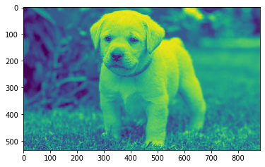
[9.09810233e-01 2.60317846e-02 1.97574078e-02 2.77915537e-02
 1.31694722e-02 2.52446879e-03 6.36716463e-04 2.17571455e-04
 6.07920241e-05 9.15640448e-01 2.48822727e-02 1.86702013e-02
 2.63437145e-02 1.18992323e-02 2.02411568e-03 4.07844204e-04
 1.09513721e-04 2.26580113e-05 9.71165298e-01 9.19026798e-03
 6.63816594e-03 8.62583483e-03 3.68366898e-03 5.02318497e-04
 1.13426757e-04 5.40127416e-05 2.70063708e-05 8.33778879e-01
 4.29548185e-02 3.26013800e-02 5.29056931e-02 2.73491801e-02
 7.36566005e-03 1.98765890e-03 8.80608375e-04 1.76121675e-04
 9.00955422e-01 2.52231333e-02 1.89294439e-02 3.21553830e-02
 1.65154923e-02 4.43605931e-03 1.16101879e-03 5.12783301e-04
 1.11264301e-04 9.08750580e-01 2.31333775e-02 1.64857417e-02
 2.92278667e-02 1.50633649e-02 4.92893055e-03 1.33347821e-03
 7.40821225e-04 3.35838955e-04]