XGBoost for Regression

XGBoost (Extreme Gradient Boosting) is an optimized and scalable implementation of the gradient boosting framework designed for supervised learning tasks such as regression and classification. In regression, XGBoost aims to predict continuous numeric values by minimizing loss functions (e.g., RMSE or MSE) while incorporating regularisation to prevent overfitting.

Use XGBoost in Regression

XGBoost is particularly effective for regression problems due to:

• Handling Missing Values: Automatically handles missing data without requiring imputation.
• Feature Importance: Provides insight into which features impact predictions.
• Scalability: Efficient on large datasets with GPU acceleration.
• Ensemble Learning: Combines multiple weak models to create a strong predictive model.

Loss Functions and Regularization

XGBoost constructs its models by minimizing an objective function that balances two aspects:

• Prediction Accuracy — measured using a loss function
• Model Complexity — controlled via regularization

Formally, the objective function is:

Obj = \sum_{i=1}^{n} L(y_i, \hat{y}_i) + \Omega(f_t)

Where:

• L(y_i,\hat y_i ) quantifies the error between actual value y_i and predicted value \hat y_i .
• \Omega(f_t) penalizes overly complex trees to avoid overfitting.

Loss Functions

XGBoost supports multiple loss functions depending on the task:

1. Regression (continuous target):

L(y_i, \hat{y}_i) = (y_i - \hat{y}_i)^2

This is also referred to as squared error loss ("reg:squarederror" in XGBoost). It penalizes larger errors more heavily, which is suitable for regression tasks where extreme deviations matter.

2. Binary Classification (0/1 target):

L(y_i, \hat{y}_i) = -[y_i \log(\hat{p}_i) + (1-y_i)\log(1-\hat{p}_i)]

This is logistic loss ("reg:logistic") and is used when predictions are probabilities between 0 and 1.

Working in Regression

1. During tree building, XGBoost calculates gain for each possible split:

Gain = \frac{1}{2} \left( \frac{(\sum_{left} g_i)^2}{\sum_{left} h_i + \lambda} + \frac{(\sum_{right} g_i)^2}{\sum_{right} h_i + \lambda} - \frac{(\sum_{total} g_i)^2}{\sum_{total} h_i + \lambda} \right) - \gamma

2. A split is accepted only if Gain > 0, ensuring that the split improves the model after considering regularization.

3. Leaf weights are calculated as:

w_j = -\frac{\sum_{i \in j} g_i}{\sum_{i \in j} h_i + \lambda}

This shows how L2 regularization (λ) shrinks leaf weights and L1 (α) further encourages zero weights.

Implementation

Step 1: Installation

Lets install the XGBoost package,

pip install --upgrade xgboost

Step 2: Importing libraries and Dataset

Here we will load seaborn and pandas library. We will use the mpg dataset from Seaborn to show the working.

import seaborn as sns
import pandas as pd

df = sns.load_dataset('mpg').dropna()

X = df.drop(columns=['mpg'])
y = df['mpg']

Step 3: Data Preprocessing

We will convert categorical features into numerical values using one-hot encoding.

X = pd.get_dummies(X, drop_first=True)

Step 4: Splitting Data

Split the data into training and testing sets where 70% data will be used for training and rest for testing.

from sklearn.model_selection import train_test_split

X_train, X_test, y_train, y_test = train_test_split(
    X, y, test_size=0.3, random_state=42)

Step 5: Training XGBoost Regressor

We will train the XGBoost Regressor.

import xgboost as xgb
from sklearn.metrics import mean_squared_error, r2_score
import numpy as np

model = xgb.XGBRegressor(objective='reg:squarederror',
                         n_estimators=100, random_state=42)
model.fit(X_train, y_train)
y_pred = model.predict(X_test)

rmse = np.sqrt(mean_squared_error(y_test, y_pred))
r2 = r2_score(y_test, y_pred)

print(f'RMSE: {rmse:.3f}')
print(f'R²: {r2:.3f}')

Output:

RMSE: 2.967
R²: 0.834

Step 6: Hyperparameter Tuning

We get optimized model performance with GridSearchCV.

from sklearn.model_selection import GridSearchCV

param_grid = {
    'max_depth': [3, 6, 9],
    'learning_rate': [0.01, 0.1, 0.2],
    'subsample': [0.8, 1.0],
    'colsample_bytree': [0.8, 1.0]
}

grid_search = GridSearchCV(
    estimator=model, param_grid=param_grid, cv=3, n_jobs=-1, verbose=1)
grid_search.fit(X_train, y_train)

print("Best parameters:", grid_search.best_params_)

Output:

Fitting 3 folds for each of 36 candidates, totalling 108 fits
Best parameters: {'colsample_bytree': 0.8, 'learning_rate': 0.1, 'max_depth': 3, 'subsample': 0.8}

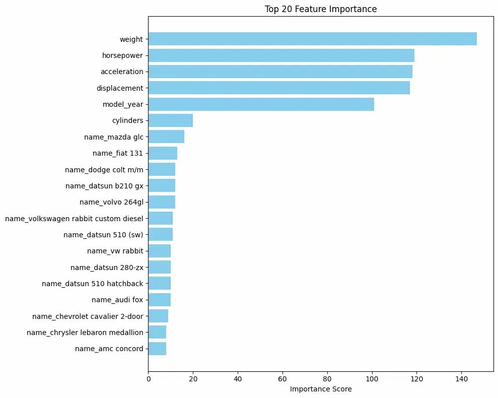
Step 7: Feature Plotting

We will plot the top important features.

import matplotlib.pyplot as plt
import pandas as pd
import numpy as np

importance = model.get_booster().get_score(importance_type='weight')

importance_df = pd.DataFrame({
    'Feature': list(importance.keys()),
    'Importance': list(importance.values())
}).sort_values(by='Importance', ascending=False)

top_n = 20
plt.figure(figsize=(10, 8))
plt.barh(
    importance_df['Feature'].head(top_n)[::-1],
    importance_df['Importance'].head(top_n)[::-1],
    color='skyblue'
)
plt.xlabel('Importance Score')
plt.title(f'Top {top_n} Feature Importance')
plt.tight_layout()
plt.show()

Output:

Limitations

• Computationally intensive: Can be slow to train on very large datasets, especially with many trees.
• Parameter tuning required: Requires careful tuning of hyperparameters (e.g., learning rate, max depth, number of estimators) for optimal performance.
• Memory consumption: Can use a lot of RAM for large datasets or deep trees.
• Less interpretable: Compared to linear regression, the final model is harder to interpret.