Contractive Autoencoder (CAE)

Contractive Autoencoder (CAE) is a type of autoencoder designed to learn robust and stable feature representations. It improves upon traditional autoencoders by adding a penalty term to the loss function, making the learned features less sensitive to small changes in the input data.

• Combines reconstruction loss with a contractive regularization term.
• Effective for feature extraction and representation learning tasks.

Loss Function of Contractive AutoEncoder

Contractive Autoencoders adds an additional penalty term to the standard autoencoder loss function:

\lVert J_h(X) \rVert_F^2 = \sum_{ij} \left( \frac{\partial h_j(X)}{\partial X_i} \right)^2

This penalty is the Frobenius norm of the encoder Jacobian, which measures how sensitive the hidden representation is to changes in the input. Minimizing this term encourages the learned features to remain stable under small input perturbations.

To compute the penalty, we first calculate the Jacobian matrix of the hidden layer with respect to the input:

\begin{aligned}Z_j &= W_i X_i \\ h_j &= \phi(Z_j)\end{aligned}

where \phi represents the activation function.

Applying the chain rule gives:

\begin{aligned}\frac{\partial h_j}{\partial X_i} &= \frac{\partial \phi(Z_j)}{\partial X_i} \\ &= \frac{\partial \phi(W_i X_i)}{\partial W_i X_i} \frac{\partial W_i X_i}{\partial X_i} \\ &= [\phi(W_i X_i)(1 - \phi(W_i X_i))] \, W_{i} \\ &= [h_j(1 - h_j)] \, W_i\end{aligned}

Unlike standard gradient computation, h(X) is treated as a vector-valued function. Therefore, each hidden unit contributes its own gradient vector, forming the Jacobian matrix.

Let \operatorname{diag}(x) denote a diagonal matrix. The Jacobian can then be written as:

\frac{\partial h}{\partial X} = diag[h(1 - h)] \, W^T

Substituting this into the penalty term and simplifying yields:

\begin{aligned}\lVert J_h(X) \rVert_F^2 &= \sum_{ij} \left( \frac{\partial h_j}{\partial X_i} \right)^2 \\[10pt] &= \sum_i \sum_j [h_j(1 - h_j)]^2 (W_{ji}^T)^2 \\[10pt] &= \sum_j [h_j(1 - h_j)]^2 \sum_i (W_{ji}^T)^2 \\[10pt]\end{aligned}

This final expression represents the contractive penalty used in the CAE loss function, encouraging the encoder to learn robust and stable feature representations.

Working

• Encode the Input: The encoder compresses the input data into a lower-dimensional latent representation.
• Apply Contractive Penalty: A penalty term based on the Jacobian of the hidden representation is added to the loss function to encourage robustness.
• Reconstruct the Input: The decoder reconstructs the original input from the latent representation.
• Optimize the Model: The model minimizes both the reconstruction error and the contractive loss during training.

Relationship with Sparse Autoencoder

Both Contractive Autoencoders (CAEs) and Sparse Autoencoders learn effective feature representations.

• Sparse Autoencoders encourage most hidden units to remain close to zero.
• This often results in small derivatives and smaller Jacobian values.
• The resulting contractive behavior is an indirect effect of sparsity.
• CAEs explicitly enforce robustness through a Jacobian-based penalty.

Thus, Sparse Autoencoders achieve contractive behavior indirectly, whereas CAEs achieve it through explicit regularization.

Relationship with Denoising Autoencoder

Both Contractive Autoencoders (CAEs) and Denoising Autoencoders (DAEs) aim to learn robust feature representations.

• Denoising Autoencoders improve robustness by reconstructing clean inputs from corrupted data.
• Contractive Autoencoders improve robustness by adding a Jacobian-based penalty that makes latent representations less sensitive to small input variations.

This highlights that DAEs achieve robustness through noise-based training, while CAEs achieve it through explicit regularization.

Implementation

Step 1: Import Required Libraries and Load the Dataset

Importing TensorFlow and loading the Fashion-MNIST dataset. The pixel values are normalized to improve training performance.

import tensorflow as tf

(x_train, _), (x_test, _) = tf.keras.datasets.fashion_mnist.load_data()
x_train = x_train.astype('float32') / 255.
x_test = x_test.astype('float32') / 255.

Step 2: Build the Contractive Autoencoder Model

Creating an autoencoder with a bottleneck layer that learns compact latent representations.

class AutoEncoder(tf.keras.Model):
    def __init__(self):
        super(AutoEncoder, self).__init__()
        self.flatten_layer  =tf.keras.layers.Flatten()
        self.dense1 = tf.keras.layers.Dense(64, activation=tf.nn.relu)
        self.dense2 = tf.keras.layers.Dense(32, activation=tf.nn.relu)
        
        
        self.bottleneck = tf.keras.layers.Dense(16, activation=tf.nn.relu)
    
        self.dense4 = tf.keras.layers.Dense(32, activation=tf.nn.relu)
        self.dense5 = tf.keras.layers.Dense(64, activation=tf.nn.relu)
        
        self.dense_final = tf.keras.layers.Dense(784)
    
    def call(self, inp):
        x_reshaped = self.flatten_layer(inp)
        x = self.dense1(x_reshaped)
        x = self.dense2(x)
        x = self.bottleneck(x)
        x_hid= x
        x = self.dense4(x)
        x = self.dense5(x)
        x = self.dense_final(x)
        return x, x_reshaped,x_hid

Step 3: Define the Contractive Loss Function

Combining the reconstruction loss with a contractive penalty to learn robust latent representations.

def loss(x, x_bar, h, model, Lambda =100):
    reconstruction_loss = tf.reduce_mean( 
                tf.keras.losses.mse(x, x_bar) 
            ) 
    reconstruction_loss *= 28 * 28
    W= tf.Variable(model.bottleneck.weights[0])
    dh = h * (1 - h)  
    W = tf.transpose(W)
    contractive = Lambda * tf.reduce_sum(tf.linalg.matmul(dh**2,
                                                          tf.square(W)),
                                         axis=1)
    total_loss = reconstruction_loss + contractive
    return total_loss

Step 4: Compute Gradients

Using TensorFlow's GradientTape to compute gradients of the total loss with respect to the trainable parameters.

def grad(model, inputs):
    with tf.GradientTape() as tape:
        reconstruction, inputs_reshaped, hidden = model(inputs)
        loss_value = loss(inputs_reshaped, reconstruction, hidden, model)
    return loss_value, tape.gradient(loss_value, model.trainable_variables), inputs_reshaped, reconstruction

Step 5: Train the model

Training the Contractive Autoencoder using the Adam optimizer to minimize the total loss.

model = AutoEncoder()
optimizer = tf.optimizers.Adam(learning_rate=0.001)
global_step = tf.Variable(0)
num_epochs = 200
batch_size = 128
for epoch in range(num_epochs):
    print("Epoch: ", epoch)
    for x in range(0, len(x_train), batch_size):
        x_inp = x_train[x : x + batch_size]
        loss_value, grads, inputs_reshaped, reconstruction = grad(model, x_inp)
        optimizer.apply_gradients(
    zip(grads, model.trainable_variables)
)
        
    print("Step: {}, Loss: {}".format(global_step.numpy(),tf.reduce_sum(loss_value)))

Output:

Epoch: 0
Step: 0, Loss: 3717.4609375
Epoch: 1
Step: 0, Loss: 3014.34912109375
Epoch: 2
Step: 0, Loss: 2702.09765625
Epoch: 3
Step: 0, Loss: 2597.461669921875
Epoch: 4
Step: 0, Loss: 2489.85693359375
Epoch: 5
Step: 0, Loss: 2351.0146484375
Epoch: 6
Step: 0, Loss: 2094.60693359375
Epoch: 7
Step: 0, Loss: 1996.68994140625
Epoch: 8
Step: 0, Loss: 1930.5377197265625
Epoch: 9
Step: 0, Loss: 1881.977294921875
...
...

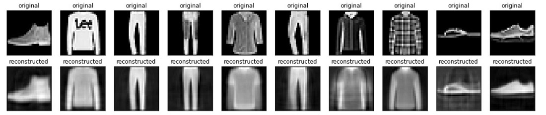
Step 6: Visualize the Reconstruction Results

Comparing original images with their reconstructed versions to evaluate the performance of the Contractive Autoencoder.

n = 10
import matplotlib.pyplot as plt
plt.figure(figsize=(20, 4))
for i in range(n):
  ax = plt.subplot(2, n, i + 1)
  plt.imshow(x_test[i])
  plt.title("original")
  plt.gray()
  ax.get_xaxis().set_visible(False)
  ax.get_yaxis().set_visible(False)

  ax = plt.subplot(2, n, i + 1 + n)
  reconstruction, inputs_reshaped,hidden = model(x_test[i].reshape((1,784)))
  plt.imshow(reconstruction.numpy().reshape((28,28)))
  plt.title("reconstructed")
  plt.gray()
  ax.get_xaxis().set_visible(False)
  ax.get_yaxis().set_visible(False)
plt.show()

Output: