Plotting Histogram in Python using Matplotlib

A histogram is used to visualize the distribution of numerical data by grouping values into intervals called bins. It helps identify the frequency of data values, making it easier to observe patterns, spread and the overall distribution of a dataset.

Example: The following example creates a simple histogram using a list of numerical values.

import matplotlib.pyplot as plt

data = [2, 3, 3, 4, 5, 5, 5, 6, 7, 8]
plt.hist(data)
plt.show()

Output

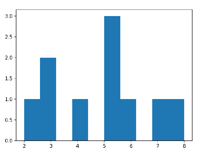
Explanation: hist() function groups the values into bins and displays the number of values that fall within each interval. By default, Matplotlib automatically determines the number of bins.

Syntax

matplotlib.pyplot.hist(x, bins=10, color=None, edgecolor=None, label=None, density=False)

Parameters:

• x: Specifies the input data to be plotted as a histogram.
• bins: Specifies the number of intervals (bins) or the bin edges used to group the data. The default value is 10.
• color: Specifies the fill color of the histogram bars.
• edgecolor: Specifies the color of the edges around each bar.
• label: Adds a label for the histogram, which can be displayed using legend().
• density: If set to True, the histogram displays probability density instead of frequency counts.

Creating a Basic Histogram

A basic histogram groups numerical data into bins and displays the frequency of values in each interval. It provides a quick overview of how the data is distributed.

import matplotlib.pyplot as plt
import numpy as np

data = np.random.randn(1000)
plt.hist(data, bins=30, color='skyblue', edgecolor='black')

plt.xlabel('Values')
plt.ylabel('Frequency')
plt.title('Basic Histogram')
plt.show()

Output

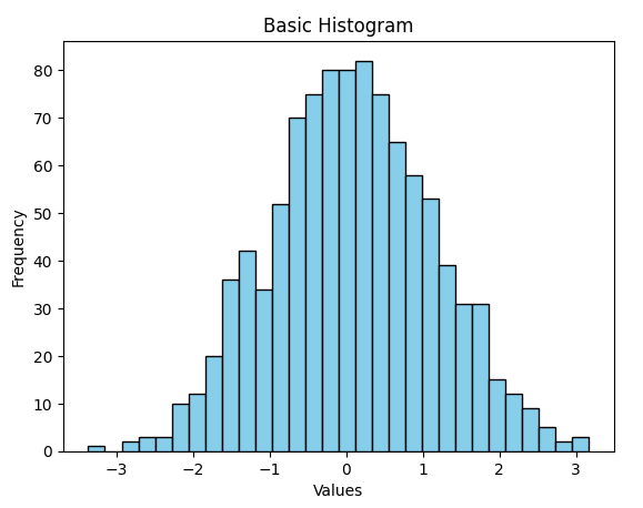
Explanation: hist() function divides the data into 30 bins and plots the frequency of values in each bin and color parameter sets the bar color to sky blue, while edgecolor adds black borders around the bars. The axis labels and title make the histogram easier to understand.

Histogram with Density Curve

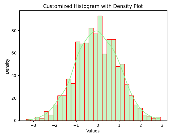
A density curve can be added to a histogram to visualize the overall distribution of the data along with the frequency of values. This provides a smoother view of the data pattern.

import matplotlib.pyplot as plt
import seaborn as sns
import numpy as np

data = np.random.randn(1000)
sns.histplot(data, bins=30, kde=True, color='lightgreen', edgecolor='red')

plt.xlabel('Values')
plt.ylabel('Density')
plt.title('Customized Histogram with Density Plot')
plt.show()

Output

Explanation:

• The histplot() function creates a histogram with 30 bins, while kde=True overlays a smooth density curve that represents the data distribution.
• The histogram bars are displayed in light green with red edges, and the axis labels and title improve the readability of the chart.

Customized Histogram

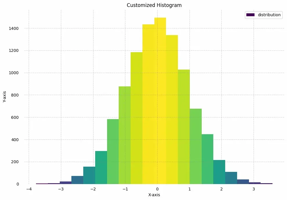
A histogram can be customized by modifying its appearance with colors, gridlines, legends and other visual elements. This helps create more informative and visually appealing charts.

import matplotlib.pyplot as plt
import numpy as np
from matplotlib import colors
from matplotlib.ticker import PercentFormatter

np.random.seed(23685752)
N_points = 10000
n_bins = 20
x = np.random.randn(N_points)
y = 0.8 ** x + np.random.randn(N_points) + 25

legend = ['distribution']
fig, axs = plt.subplots(1, 1, figsize=(10, 7), tight_layout=True)

for s in ['top', 'bottom', 'left', 'right']:
    axs.spines[s].set_visible(False)

axs.xaxis.set_ticks_position('none')
axs.yaxis.set_ticks_position('none')
axs.xaxis.set_tick_params(pad=5)
axs.yaxis.set_tick_params(pad=10)
axs.grid(visible=True, color='grey', linestyle='-.', linewidth=0.5, alpha=0.6)

fig.text(0.9, 0.15, 'Jeeteshgavande30',
         fontsize=12,
         color='red',
         ha='right',
         va='bottom',
         alpha=0.7)

N, bins, patches = axs.hist(x, bins=n_bins)
fracs = ((N ** (1 / 5)) / N.max())
norm = colors.Normalize(fracs.min(), fracs.max())

for thisfrac, thispatch in zip(fracs, patches):
    color = plt.cm.viridis(norm(thisfrac))
    thispatch.set_facecolor(color)

plt.xlabel("X-axis")
plt.ylabel("Y-axis")
plt.legend(legend)
plt.title('Customized Histogram with Watermark')
plt.show()

Output

Explanation:

• This example generates a histogram with 20 bins and applies a Viridis color gradient to the bars based on their frequencies.
• The chart is further customized by removing the axis borders and tick marks, adding gridlines, placing a text watermark, and including axis labels, a legend and a title to improve the overall presentation.

Multiple Histograms Using Subplots

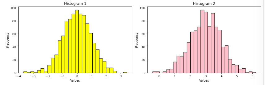
Subplots allow multiple histograms to be displayed in a single figure. This makes it easier to compare the distribution of different datasets side by side.

import matplotlib.pyplot as plt
import numpy as np

data1 = np.random.randn(1000)
data2 = np.random.normal(loc=3, scale=1, size=1000)
fig, axes = plt.subplots(nrows=1, ncols=2, figsize=(12, 4))

axes[0].hist(data1, bins=30, color='Yellow', edgecolor='black')
axes[0].set_title('Histogram 1')
axes[1].hist(data2, bins=30, color='Pink', edgecolor='black')
axes[1].set_title('Histogram 2')

for ax in axes:
    ax.set_xlabel('Values')
    ax.set_ylabel('Frequency')

plt.tight_layout()
plt.show()

Output

Explanation:

• The subplots() function creates two plotting areas within the same figure. Each histogram is plotted separately with 30 bins using different colors.
• Titles and axis labels are added to both plots, while tight_layout() automatically adjusts the spacing to prevent overlapping elements.

Stacked Histogram

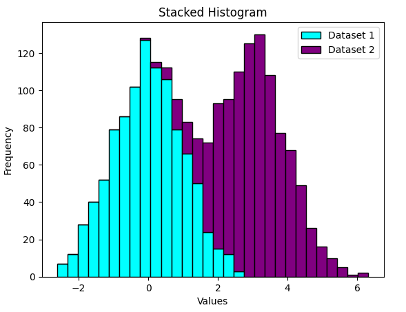
A stacked histogram displays multiple datasets in the same histogram by stacking their frequencies on top of each other. This helps compare the overall distribution and contribution of each dataset.

import matplotlib.pyplot as plt
import numpy as np

data1 = np.random.randn(1000)
data2 = np.random.normal(loc=3, scale=1, size=1000)

plt.hist([data1, data2], bins=30, stacked=True, color=['cyan', 'Purple'], edgecolor='black')
plt.xlabel('Values')
plt.ylabel('Frequency')
plt.title('Stacked Histogram')
plt.legend(['Dataset 1', 'Dataset 2'])
plt.show()

Output

Explanation:

• The hist() function plots both datasets together using 30 bins. Setting stacked=True stacks the frequencies of the datasets into a single histogram.
• Different colors distinguish the datasets, while the axis labels, title and legend make the visualization easier to interpret.

2D Histogram (Hexbin Plot)

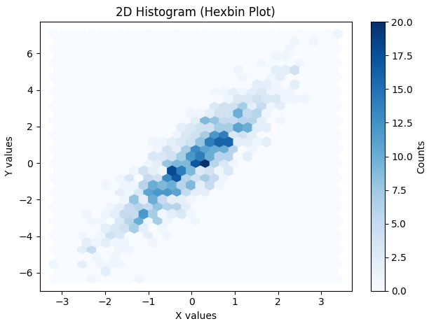
A 2D histogram groups data into hexagonal bins to show the density of points across two variables. It is useful for visualizing large datasets where many points overlap in a scatter plot.

import matplotlib.pyplot as plt
import numpy as np

x = np.random.randn(1000)
y = 2 * x + np.random.normal(size=1000)

plt.hexbin(x, y, gridsize=30, cmap='Blues')
plt.xlabel('X values')
plt.ylabel('Y values')
plt.title('2D Histogram (Hexbin Plot)')
plt.colorbar(label='Counts')
plt.show()

Output

Explanation:

• The hexbin() function divides the plot into hexagonal bins and counts the number of data points in each bin.
• The gridsize parameter controls the number of hexagons, while the cmap parameter applies a blue color gradient to represent data density.
• The colorbar indicates the number of points contained in each hexagonal bin.