

State Space Search is used to solve problems by finding different possible states and their transitions. In simple terms it’s like finding the best route to goal by trying different paths.
- It works by systematically checking possible states until the goal is reached.
- This method can be applied to various AI tasks such as pathfinding, puzzle solving, game playing and more.
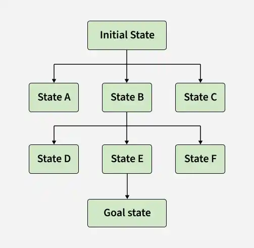
- Nodes represent possible states of the problem.
- Edges represent actions or transitions between states.
Terminologies
- State: A specific configuration of the problem.
- Initial State: Starting point of the search.
- Goal State: Desired end configuration.
- Transition: An action that changes one state to another.
- Path: A sequence of states connected by transitions.
- Search Strategy: Method used to explore the state space.
Features
- Branching Factor: Average number of successors per state. A higher branching factor makes search tree wider which increases time and resources required.
- Depth: Number of steps from the initial state to the goal state. Deeper trees increase the search time as more states must be explored.
- Completeness: A search is complete if it guarantees finding a solution if one exists. It ensures the algorithm will eventually reach the goal.
- Optimality: A search is optimal if it guarantees finding the best solution, according to a specific criterion liked least cost or shortest path.
- Time and Space Complexity: Measure the time and memory required for the search, both of which increase with the branching factor and search depth.
Steps in State Space Search
Step 1: Define the State Space
Identify all possible states and their transitions. To do this model the problem in a way that includes all relevant configurations and actions.
Step 2: Pick a Search Strategy
Choose a method for exploring the state space. Search strategies can be broadly classified into Uninformed Search and Informed Search based on whether they use additional knowledge about the problem to guide the search.
1. Uninformed Search
Uninformed search strategies explore the state space without using heuristic information about how close a state is to the goal. Common strategies include:
- Breadth-First Search (BFS): Explores all nodes at one depth level before moving to the next, ideal for unweighted graphs.
- Depth-First Search (DFS): Explores a branch as deeply as possible before backtracking. It uses less memory but may not guarantee completeness or optimality.
- Uniform Cost Search (UCS): Expands the least costly node first which ensures the lowest-cost solution.
2. Informed Search
Informed search strategies use heuristic information to guide the search toward the goal more efficiently. Common strategies include:
- Greedy Best-First Search: Expands nodes that appear closest to the goal based on a heuristic.
- A* Search Algorithm: Combines path cost and heuristic to guarantee completeness and optimality.
Admissible Heuristic: A heuristic is admissible if it never overestimates the actual cost of reaching the goal. A* is optimal when it uses an admissible heuristic.
Step 3: Start the Search and Extend the Nodes
Add the initial state and begin the search. The selected search strategy expands nodes, generates successor states and adds them to the frontier. If a state matches the goal, the algorithm retraces the path to the solution and stops the search.
Step 4: Address State Repetition
Prevent revisiting same state by tracking visited states helps in avoiding cycles and unnecessary exploration.
Step 5: End the Search
The search ends when goal state is found or when all states have been explored without finding a solution.
Example: BFS algorithm on 8-Puzzle Problem
The 8-puzzle is a sliding puzzle with a 3×3 grid containing 8 numbered tiles and one blank space. The goal is to arrange the tiles from 1 to 8 in order, with the blank space in the lower-right corner, using the minimum number of moves.
Here's an explanation of how the BFS algorithm works to explore the state space and find the solution in the following scenario:
- States: Each arrangement of the 3x3 grid consisting of tiles numbered 1 through 8 and a blank space.
- Initial State: A specific tile layout at the start.
- Goal State: Arrangements with blank space in the lower-right corner and the tiles arranged in numerical order.
- Actions: Up, down, left or right movement of the empty space.
- Transition Model: Describes the state generated after performing an action.
- Path Cost: Cost of each move is uniform and equals one.
Step 1: Load Dependencies
The required libraries are imported for array manipulation, visualization and implementing the BFS queue.
import numpy as np
import matplotlib.pyplot as plt
from queue import Queue
Step 2: Visualization Function
Using matplotlib to create a grid for each state in the path and display the tile arrangements. This helps visualize the solution path from the initial state to the goal state.
- fig, axes = plt.subplots(...): Creates subplots for displaying the puzzle states.
- ax.imshow(...): Displays each puzzle state as a grid.
- ax.text(...): Displays the tile numbers while keeping the blank space empty.
def visualize_puzzle(path):
    fig, axes = plt.subplots(nrows=len(path), ncols=1,
                             figsize=(3, 3 * len(path)))
    if len(path) == 1:
        axes = [axes]
    for ax, state in zip(axes, path):
        ax.imshow(state, cmap='tab20', vmin=0, vmax=9)
        ax.set_xticks(np.arange(3))
        ax.set_yticks(np.arange(3))
        ax.set_xticklabels([])
        ax.set_yticklabels([])
        for i in range(3):
            for j in range(3):
                ax.text(j, i, state[i, j] if state[i, j] != 0 else '',
                        ha='center', va='center', color='white', fontsize=20)
        ax.grid(color='black')
    plt.tight_layout()
    plt.show()
Step 3: BFS Algorithm
BFS starts with the initial state and explores the state space level by level using a queue.
- queue.put((initial_state, [initial_state])): Adds the initial state and its path to the queue.
- visited.add(...): Stores the initial state to prevent it from being explored again.
- current_state, path = queue.get(): Retrieves the next state and its path from the queue.
def bfs_solve(initial_state, goal_state):

    queue = Queue()
    queue.put((initial_state, [initial_state]))
    visited = set()
    visited.add(tuple(initial_state.reshape(-1)))

    while not queue.empty():
        current_state, path = queue.get()
        if np.array_equal(current_state, goal_state):
            return path

        zero_pos = tuple(np.argwhere(current_state == 0)[0])
        moves = [(-1, 0), (1, 0), (0, -1), (0, 1)]
Step 4: Movement Logic
This part generates new states by moving the blank space in each valid direction.
- new_pos = (...): Calculates the new position of the blank space.
- new_state[zero_pos], new_state[new_pos] = ...: Swaps the blank space with the adjacent tile to generate a new state.
- queue.put(...): Adds an unvisited state and its path to the queue.
for move in moves:
    new_pos = (zero_pos[0] + move[0], zero_pos[1] + move[1])
    if 0 <= new_pos[0] < 3 and 0 <= new_pos[1] < 3:
        new_state = np.copy(current_state)
        new_state[zero_pos], new_state[new_pos] = new_state[new_pos], new_state[zero_pos]
        new_state_tuple = tuple(new_state.reshape(-1))
        if new_state_tuple not in visited:
            visited.add(new_state_tuple)
            queue.put((new_state, path + [new_state]))
Step 5: Main Execution
Here we define the initial and goal states and run the BFS algorithm.
- initial_state: Defines the starting arrangement of the puzzle.
- goal_state: Defines the desired arrangement of the puzzle.
initial_state = np.array([[1, 2, 3], [4, 5, 6], [0, 7, 8]])
goal_state = np.array([[1, 2, 3], [4, 5, 6], [7, 8, 0]])
solution_path = bfs_solve(initial_state, goal_state)
if solution_path:
    visualize_puzzle(solution_path)
else:
    print("No solution found.")
Output:
.png)
You can download the source code from here.
Applications
- Pathfinding: Finding the best pathways using algorithms such as A* in robotics and GPS.
- Puzzle solving: Resolving puzzles like Rubik's Cube, Sudoku and the 8-puzzle.
- AI for gaming: To identify good moves in board games like chess, checkers and others.
- Planning: Automated scheduling of tasks in logistics and robotics to achieve a specific objective.
- Natural language processing: It involves computer translation and sentence parsing by examining many interpretations.
Challenges
- Complexity: High branching factors can cause an exponential growth in the number of states to be explored.
- Resource Limitations: Memory and processing power limit size of the state space that can be practically searched.
- Quality of Heuristics: The effectiveness of the search is limited by the quality of the heuristic function.
