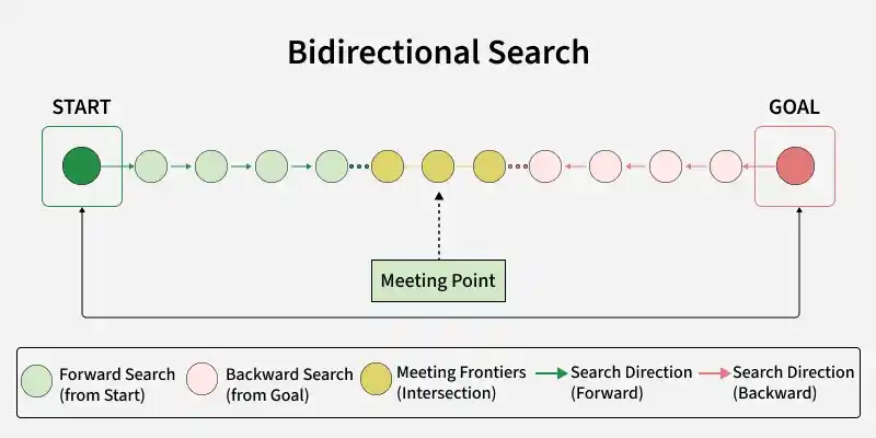
Bidirectional Search in AI

Bidirectional Search is a search technique that explores a problem from both the initial state and the goal state simultaneously.

• Dual Direction: Runs two searches that expand toward each other instead of searching entirely from one direction.
• Path Combination: Combines the paths from both sides to form a solution as soon as the two searches meet.
• Efficiency & Optimality: Finds a shortest path on an unweighted graph using Bidirectional Breadth-First Search (BFS) while potentially exploring far fewer nodes than standard BFS.

Working

Bidirectional Search maintains two search frontiers:

• Forward Search: Starts from the initial state and moves toward the goal.
• Backward Search: Starts from the goal and moves toward the initial state.
• Frontier Expansion: Both searches expand their nodes level by level.
• Intersection Check: After each expansion, the algorithm checks whether the two searches have reached a common node.
• Path Construction: When they meet, the paths from the start and goal are combined to form the final path.

The basic idea is:

Start → → → Meeting Point ← ← ← Goal

Example: Bidirectional Search for Maze Navigation

Consider a maze where:

• 0 represents an open cell.
• 1 represents a wall.
• The search starts at (0, 0).
• The goal is at (4, 4).

The algorithm runs BFS from both positions and stops when the two searches meet.

Step 1: Import Necessary Libraries

import matplotlib.pyplot as plt
import numpy as np
from collections import deque

• matplotlib is used to visualize the maze and final path.
• numpy is used to handle the maze as an array.
• deque provides an efficient queue for BFS operations.

Step 2: Define a Function to Check Valid Moves

def is_valid_move(row, col, maze):
    return (
        0 <= row < len(maze)
        and 0 <= col < len(maze[0])
        and maze[row][col] == 0
    )

• Checks whether a cell is within the maze boundaries and is not a wall.
• Returns True if the cell can be explored.

Step 3: Expand One BFS Frontier

def expand_frontier(queue, visited, parent, other_visited, maze):
    for _ in range(len(queue)):
        row, col = queue.popleft()

        for dr, dc in [(-1, 0), (1, 0), (0, -1), (0, 1)]:
            next_cell = (row + dr, col + dc)

            if is_valid_move(*next_cell, maze) and next_cell not in visited:
                visited.add(next_cell)
                parent[next_cell] = (row, col)

                if next_cell in other_visited:
                    return next_cell

                queue.append(next_cell)

    return None

• Expands one BFS level by checking the four possible movements.
• Tracks visited cells, stores parent links and checks whether the searches have met.
• Returns the meeting point when an intersection is found.

Step 4: Implement Bidirectional Search

def bidirectional_search(maze, start, goal):
    if not is_valid_move(*start, maze) or not is_valid_move(*goal, maze):
        return None, None, None

    if start == goal:
        return start, {start: None}, {goal: None}

    queue_start = deque([start])
    queue_goal = deque([goal])

    visited_start = {start}
    visited_goal = {goal}

    parent_start = {start: None}
    parent_goal = {goal: None}

    while queue_start and queue_goal:
        meeting_node = expand_frontier(
            queue_start,
            visited_start,
            parent_start,
            visited_goal,
            maze
        )

        if meeting_node is not None:
            return meeting_node, parent_start, parent_goal

        meeting_node = expand_frontier(
            queue_goal,
            visited_goal,
            parent_goal,
            visited_start,
            maze
        )

        if meeting_node is not None:
            return meeting_node, parent_start, parent_goal

    return None, None, None

• Initializes separate queues, visited sets and parent mappings for the forward and backward searches.
• Expands one BFS level from each side and checks for an intersection.
• Returns the meeting node and parent mappings when the searches meet; otherwise returns None.

Since both searches expand level by level in this unweighted maze, the resulting path is a shortest path.

Step 5: Reconstruct the Path

def reconstruct_path(meeting_node, parent_start, parent_goal):
    if meeting_node is None:
        return []

    path = []
    current = meeting_node

    while current is not None:
        path.append(current)
        current = parent_start[current]

    path.reverse()

    current = parent_goal[meeting_node]

    while current is not None:
        path.append(current)
        current = parent_goal[current]

    return path

• Traces parent links from the meeting point to the start and goal.
• Combines both parts to form the complete path without duplicating the meeting point.

Step 6: Visualize the Maze and the Path

def visualize(maze, path, start, goal):
    maze_array = np.array(maze)

    fig, ax = plt.subplots(figsize=(8, 8))

    for row in range(len(maze)):
        for col in range(len(maze[0])):
            if maze_array[row, col] == 1:
                ax.fill_between(
                    [col, col + 1],
                    row,
                    row + 1,
                    color="black"
                )

    if path:
        for row, col in path:
            ax.fill_between(
                [col, col + 1],
                row,
                row + 1,
                color="gold",
                alpha=0.6
            )

    start_row, start_col = start
    goal_row, goal_col = goal

    ax.plot(start_col + 0.5, start_row + 0.5, "go")
    ax.plot(goal_col + 0.5, goal_row + 0.5, "ro")

    ax.set_xlim(0, len(maze[0]))
    ax.set_ylim(0, len(maze))
    ax.set_xticks(range(len(maze[0]) + 1))
    ax.set_yticks(range(len(maze) + 1))
    ax.grid(True)
    ax.invert_yaxis()
    ax.xaxis.tick_top()

    plt.show()

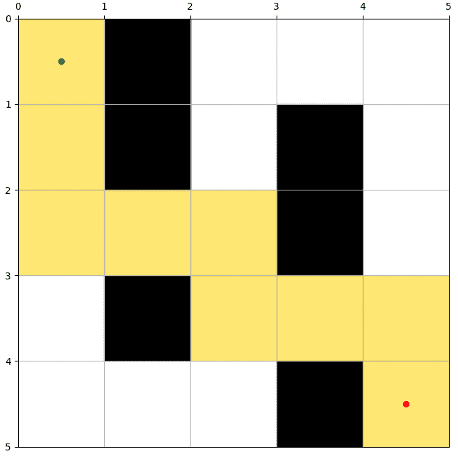
• Converts the maze into a NumPy array and displays walls as filled cells.
• Highlights the path and marks the start and goal positions.
• Configures the grid to match the maze layout.

Step 7: Define the Maze, Start and Goal

maze = [
    [0, 1, 0, 0, 0],
    [0, 1, 0, 1, 0],
    [0, 0, 0, 1, 0],
    [0, 1, 0, 0, 0],
    [0, 0, 0, 1, 0]
]

start = (0, 0)
goal = (4, 4)

• Defines the maze using 0 for open cells and 1 for walls.
• Sets (0,0) as the start and (4,4) as the goal.

Step 8: Run the Search and Visualize the Result

meeting_node, parent_start, parent_goal = bidirectional_search(
    maze,
    start,
    goal
)

path = reconstruct_path(
    meeting_node,
    parent_start,
    parent_goal
)

visualize(
    maze,
    path,
    start,
    goal
)

• Runs Bidirectional BFS and finds the meeting point.
• Reconstructs the path and visualizes the result.

Output:

You can download the source code from here.

Applications

1. Pathfinding and Route Planning: Finding paths between two known locations in maps and other graph-based environments.
2. Robotic Navigation: Planning a route between known start and target positions while reducing unnecessary exploration.
3. Puzzle Solving: Searching from both the initial and goal configurations in problems with clearly defined states.
4. Network Search: Finding short paths between two known nodes in large networks.
5. AI Planning: Reducing the search space in planning problems where both initial and goal states can be represented.

Benefits

• Reduced Search Space: Searching from both ends can significantly reduce the number of nodes explored.
• Faster Search: For suitable problems, bidirectional BFS can be much faster than one-directional BFS.
• Shortest Path: Bidirectional BFS finds a shortest path in an unweighted graph.
• Goal-Directed: Knowing both the start and goal allows the search to focus from both directions.

Challenges

• Requires a Known Goal: Both the initial and goal states must be known and backward search must be feasible.
• Not Always Faster: Its effectiveness depends on the search space and how well the two searches meet.
• Memory Usage: Both search frontiers, visited nodes and parent mappings must be maintained, which can require substantial memory for large search spaces.
• Additional Bookkeeping: Managing two searches and combining their paths adds implementation