Mixed Integer Linear Programming: Formal definition and solution space
Theoretical foundations on how MILP is defined and how its solution space looks like visually
Theoretical foundations on how MILP is defined and how its solution space looks like visually

This post is a continuation of the series (previous post) on the theory and applications of Mixed Integer Linear Programming (MILP). Today, we look at
the formal, general definition of MILP,
how its space of feasible solutions looks like.
The first part describes how MILP models look in general, what are and are not valid MILP expressions. The second part shows a little bit of theory behind MILP, which will be useful in the future posts when we will be talking about the actual algorithm for solving MILP.
This is quite a long post, so grab a coffee and dive in!
Formal definition of Mixed Integer Linear Programming
In the following text, I will use upper-case bold letters (e.g., A, E) for matrices and lower-case bold letters for vectors (e.g., x, y). MILP is an optimisation problem that can be formulated in matrix notation as follows
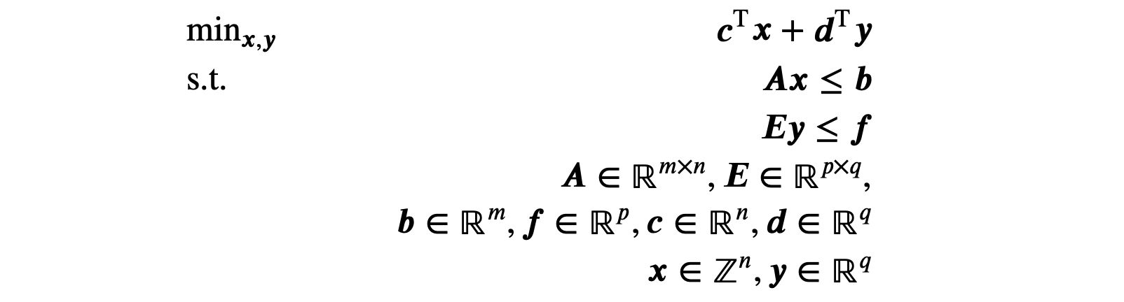
Lets break this monster down. We are given a problem instance represented by matrices and vectors A, E, b, f, c, d from various domains (ℝ stands for a set of real numbers and ℤ for a set of integer numbers). For example, if we return to our budget problem from the first post, the problem instance represents assets, their costs, estimated profits and also the budget. We say that integer vector x and continuous vector y are a feasible solution to the given problem instance, if the following conditions holds

By writing these conditions component-wise, we get

where 𝒂ᵢ are the rows of matrix A **** and 𝒆ᵢ are the rows of matrix E. These inequalities are called constraints.
In MILP, we are looking for a feasible solution x, y which minimises the objective function

If such a solution exists, we call it an optimal solution. In case you are wondering, it is possible to maximise the objective function instead; just multiply it with -1 and minimise the resulting expression. There is no guarantee that a feasible solution (let alone optimal) exists, but lets defer the discussion about these situations to the later section.
Although the matrix form is a canonical way how MILP problems are defined, model designers usually do not use it as it is very cumbersome. Instead, in practice we define constraints and objective functions using simple mathematical expressions, which will be converted internally by the solver to the matrix form (which is actually very handy for a machine). To get a feel what is correct MILP formulation and what is not, here is a list of a few examples:
𝑎₁𝑥₁ + 𝑎₂ + 𝑥₃ ≥ 𝑏₁ + 𝑎₄𝑥₄ is a correct MILP constraint. Notice that in comparison to the canonical form, the inequality is reversed, a constant is included in the left hand side and I added a variable to the right hand side. In a canonical form, this constraint would be transformed to −𝑎₁𝑥₁ − 𝑥₃ + 𝑎₄𝑥₄ ≤ −𝑏₁ + 𝑎₂ .
𝑥₁𝑥₂ is not a correct MILP expression as it is a multiplication of two variables, which is not a linear expression. The same goes for |𝑥₁|, max(𝑥₁, 𝑥₂), log(𝑥₁), etc. All of those expressions are not linear, although some of them can be linear_ised throu_gh various tricks, but more on that in another post.
𝑎₁𝑎₂ is a correct MILP expression as multiplying two fixed parameters together would result in a single fixed parameter in "compile" time, i.e., during building the matrix model but before starting the solver. Expressions where fixed parameters are transformed by a mathematical functions (such as logarithm) are also correct MILP expressions.
𝑎ₓ is not a correct MILP expression. We cannot use a variable as an index.
𝑎₁𝑥₁ < 𝑏₁ is not a correct MILP constraint, it is not possible to force strict inequality.
We finish this section by showing a MILP formulation of the budget problem from the previous post in a matrix form.
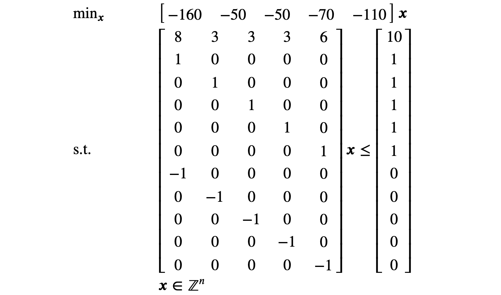
The objective uses the multiplication by -1 trick to maximise the expected profit. The budget constraint is encoded in the first row of the constraint matrix and the remaining rows correspond to constraints 0 ≤ 𝑥ᵢ, 𝑥ᵢ ≤ 1 on each variable 𝑥ᵢ (i.e., 𝑥ᵢ is required to be binary). Many solvers allow to specify the domain of the variables directly, so usually there is no need create such constraints by hand. Also, notice that our model includes only integer variables (there is no y variable), thus it is an integer linear program.
Solution space
When we know how the space of feasible solutions of MILP models looks like, we may start to reason about the general algorithm for MILP, its theoretical properties and possibly how to make more performant models.
Lets start with the following MILP model. For simplicity, we will consider only two integer variables 𝑥₁, 𝑥₂.
How can we visualise this model graphically? We start by empty 2D graph representing a model with no constraint. Gradually, we add constraint by constraint until we have a full model. In the graph, the horizontal and vertical axes correspond to values of 𝑥₁ and 𝑥₂, respectively.
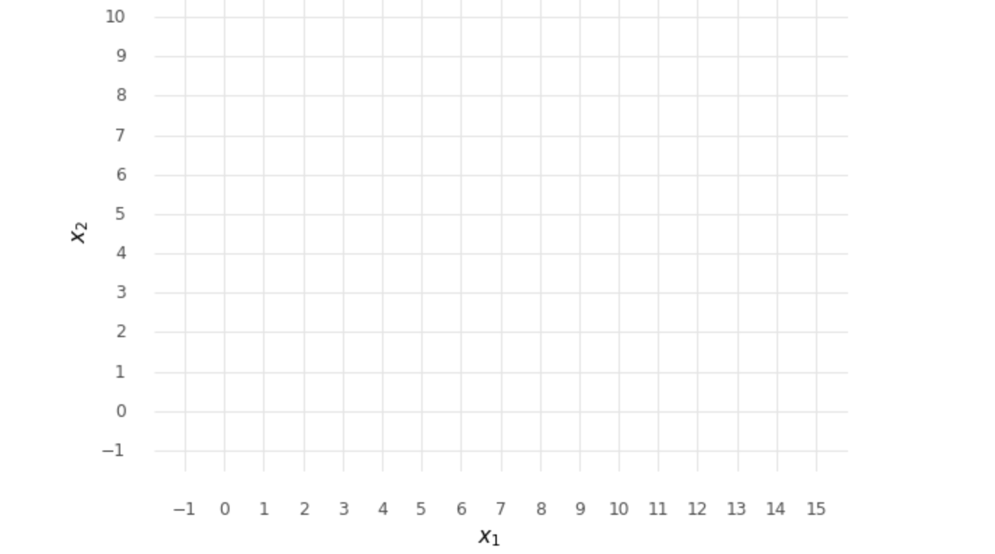
As there is currently no constraint in the model, every combination of 𝑥₁, 𝑥₂ is a feasible solution. Lets add a first constraint 4𝑥₁ ≥ 2𝑥₂ and see what happens. First, draw a line 4𝑥₁ = 2𝑥₂ in the solution space.
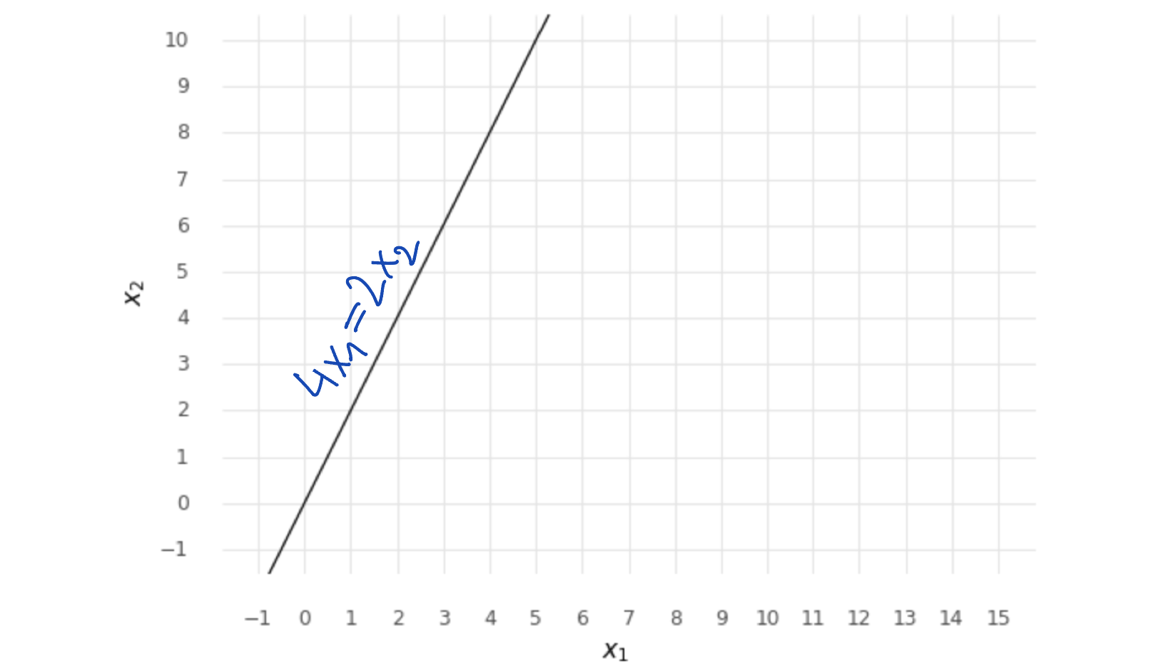
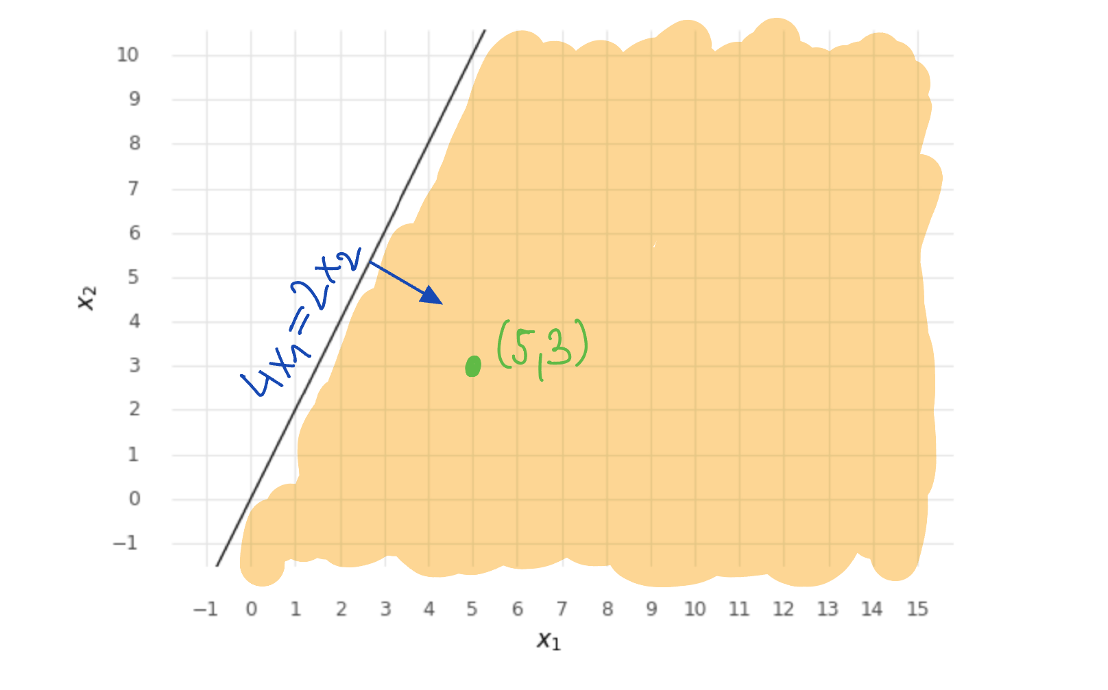
This line is a boundary between two half-spaces defined by the following inequalities: 4𝑥₁ > 2𝑥₂ and 4𝑥₁ < 2𝑥₂. All the points on one side of the line satisfy inequality 4𝑥₁ > 2𝑥₂ and all the points on the other side of line satisfy inequality 4𝑥₁ < 2𝑥₂. When I want to know which half-space represents a specific constraint, I will pick some random point 𝑥₁, 𝑥₂ that does not lie on the line, substitute it into the constraint, and check whether the constraint is satisfied. If yes, then the half-space containing this point is the one that corresponds to the constraint. If not, then the other half-space is the correct one.
So as an example, lets pick point 𝑥₁ = 5, 𝑥₂ = 3. Substitute the values into constraint

and we see that the constraint is satisfied. Therefore, the half-space containing this point is the one where all the points satisfy this constraint. In the graphs I will denote the half-space satisfying a constraint by an arrow. Of course, the points on the line also satisfy the constraint so a constraint is represented by both a boundary line and a half-space.
Lets add another constraint −2𝑥₁ + 30 ≥ 2𝑥₂. Again, we start by drawing a boundary line −2𝑥₁ + 30 = 2𝑥₂.
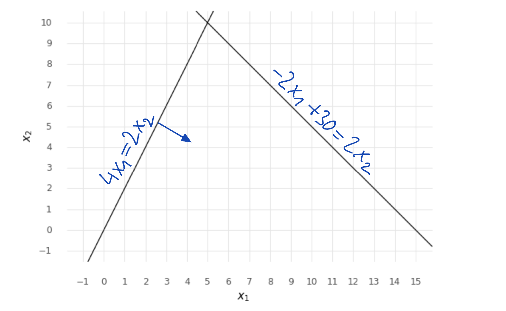
Which half-space satisfies this constraint? For this test, we pick a point 𝑥₁ = 14, 𝑥₂= 6 and substitute it into the constraint

We see that the selected point does not satisfy the constraint −2𝑥₁ + 30 ≥ 2𝑥₂ so the feasible half-space must be the other one then the one containing point 𝑥₁ = 14, 𝑥₂= 6 .
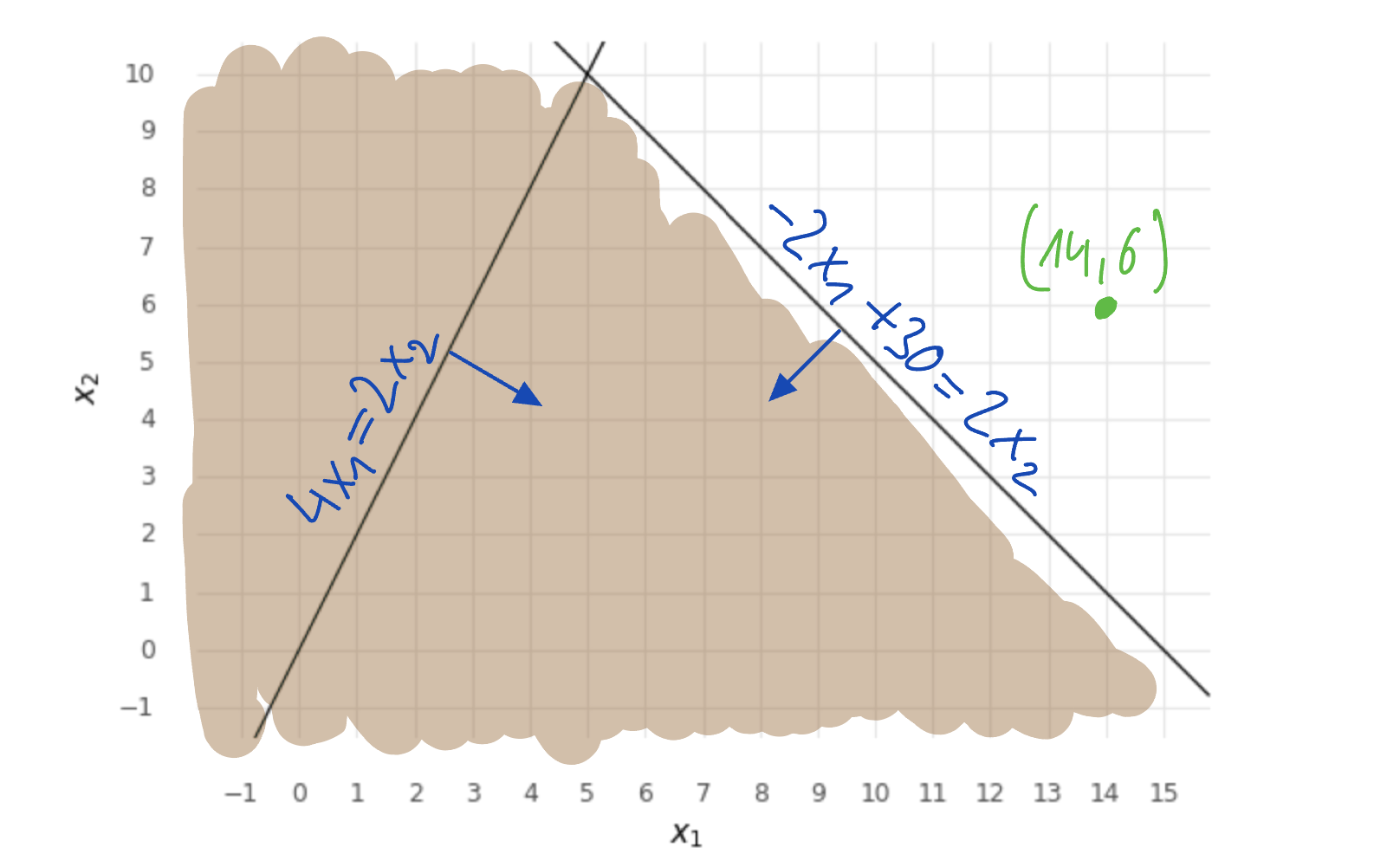
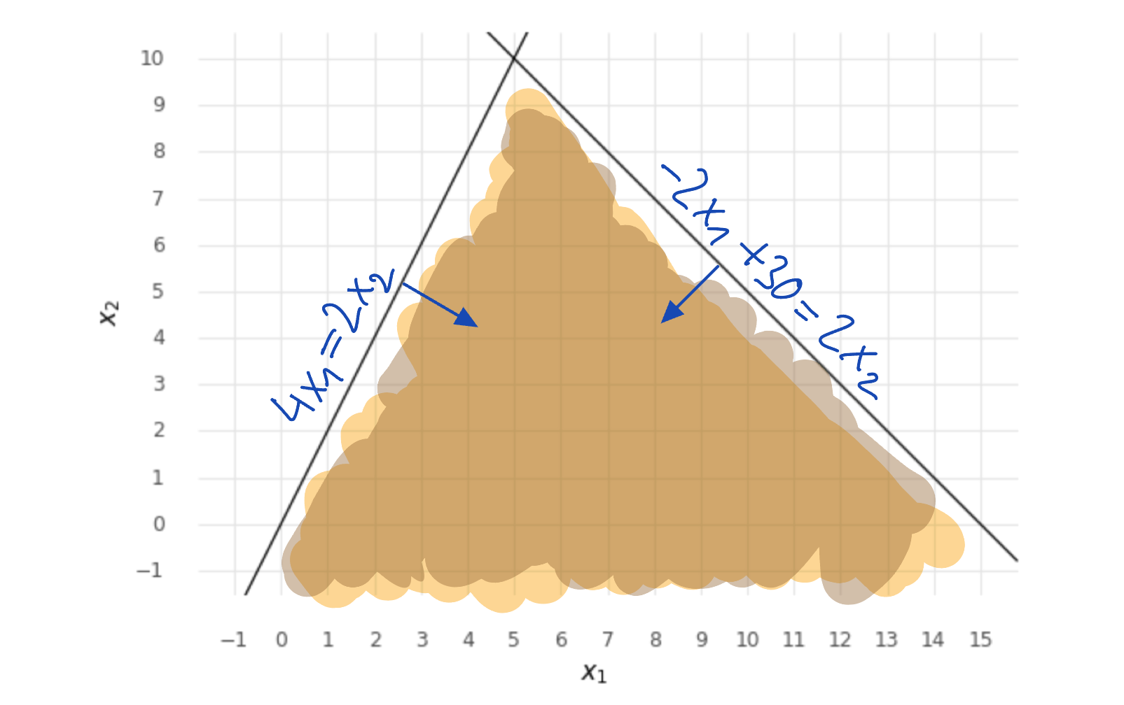
However, now as we have two constraints in the model, the feasible solution space is an intersection of the feasible half-spaces of each constraint. The reason is that we want all the constraints to be satisfied so only the solutions that lie in all feasible half-spaces are also feasible in the whole model.
Now it should be clear how to proceed with constraints 𝑥₂ ≥ 0, 0.5𝑥₁ + 3.75 ≥ 𝑥₂, so I will just draw the new feasible solution space.
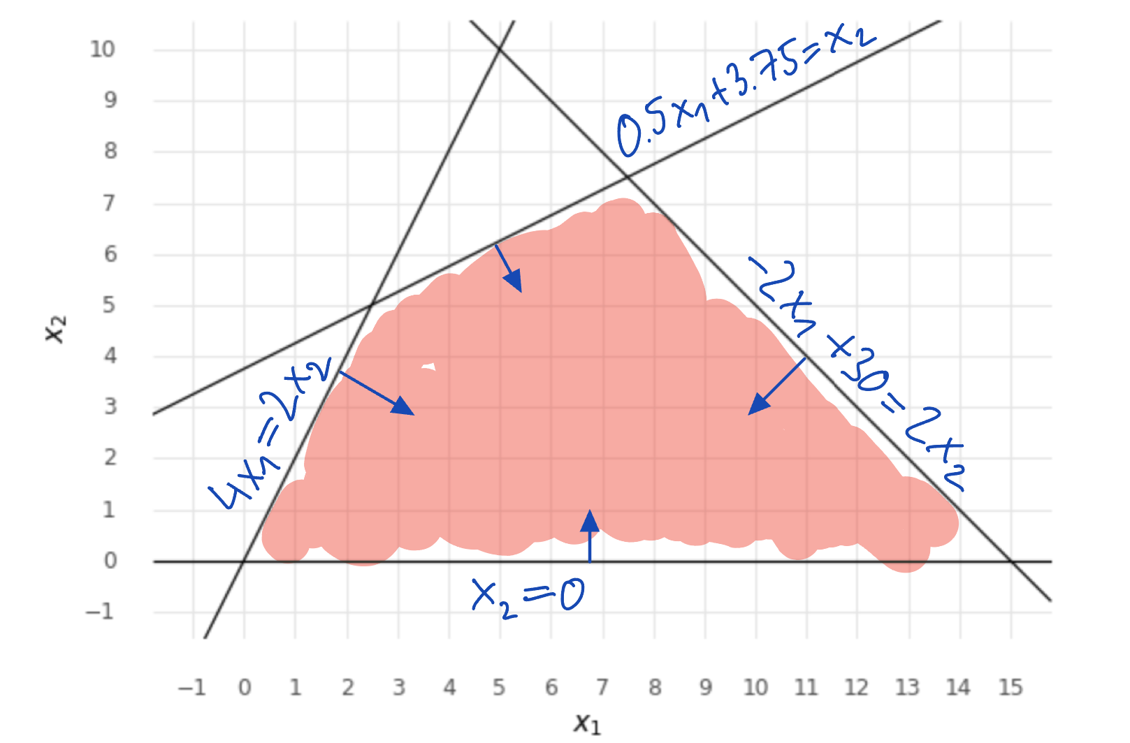
There is one thing left and that is the integrality constraint 𝑥₁, 𝑥₂ ∈ ℤ that we silently ignored at the beginning. What does this constraint mean? Simply, not all points from the coloured region are actually feasible, but only those where both 𝑥₁, 𝑥₂ are integers. We can visualise them by a grid, thus, the final feasible solution space of the example MILP model looks like this.
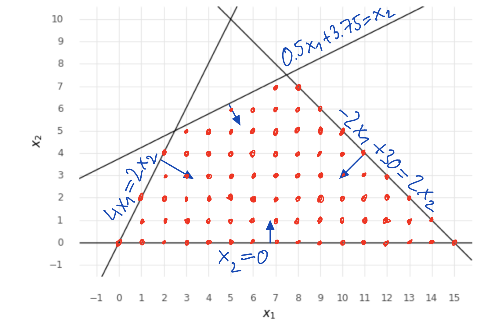
Each of those red points correspond to one feasible integer solution which satisfy all the constraints. Now, the last question is: which of those points optimise our objective function, i.e., which point gives us the smallest value of −2𝑥₁ − 3𝑥₂? This question is little bit more involved. We could extend our graph to a third dimension representing the values of the objective function, project the feasible solutions to a plane of our objective function and find the projected point that is the lowest. However, I think that it is a nice mental exercise to stay in 2D space and find the optimum there.
Many of you are probably familiar with the concept of a gradient, as it is a backbone of many ML training algorithms. In short, a gradient of a function represents a direction of the largest increase of that function at some point. That is, if we move along the gradient, we will increase the function. Knowing the gradient of the MILP's objective function tells us where to look for the optimal feasible solution. So, lets find the gradient of our objective function, which we obtain by taking the partial derivatives by each variable 𝑥₁, 𝑥₂

Since our objective function is linear, its gradient is the same for every point in the solution space. And since gradient is a direction, we can draw a vector into our solution space to show the direction of the increase in the objective function.
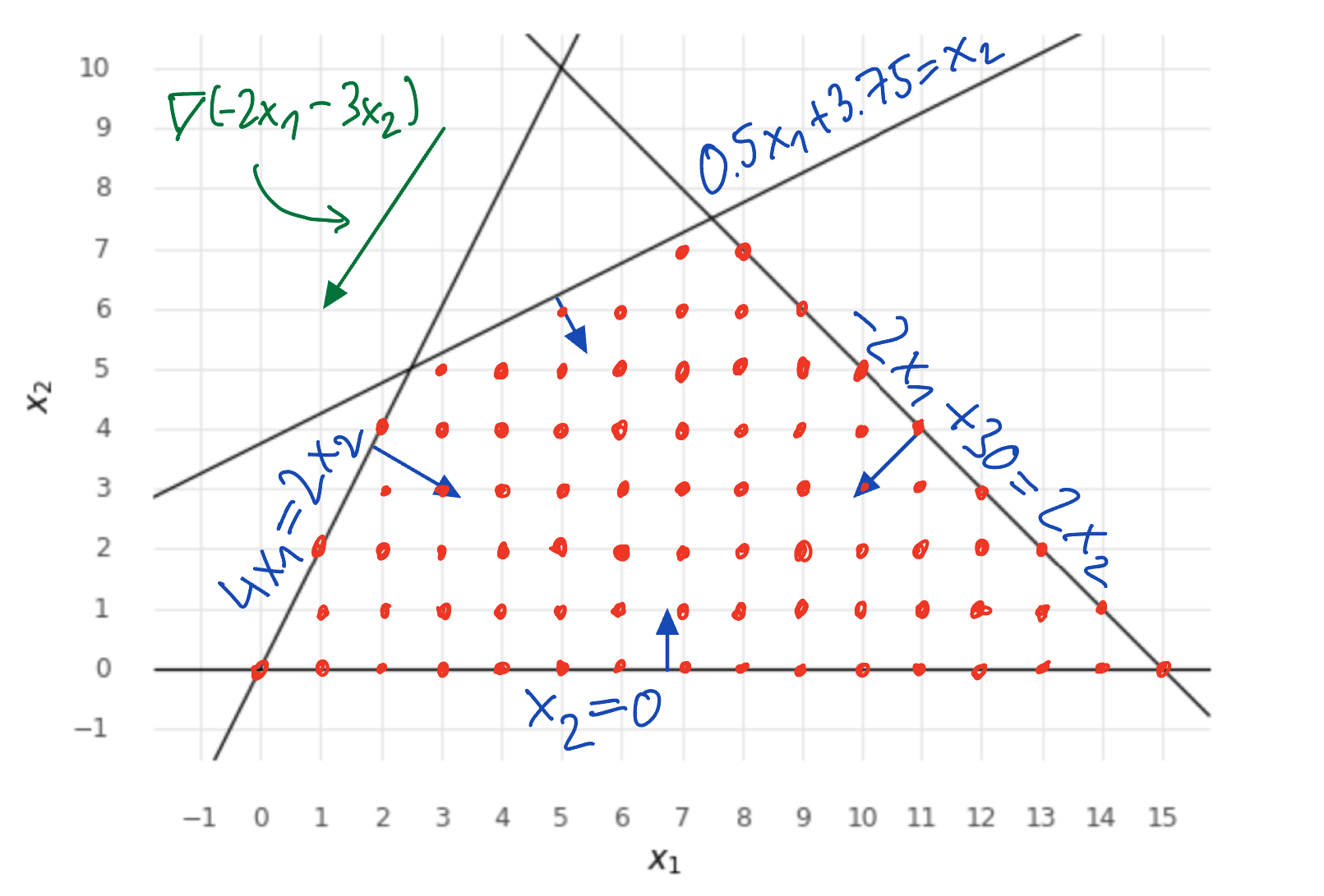
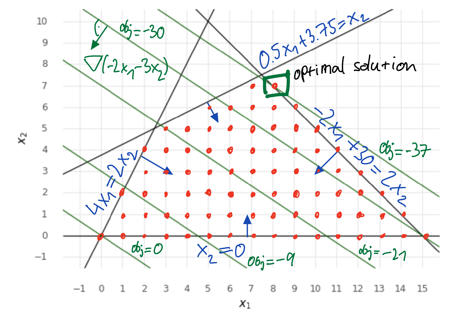
Lets draw a contour lines of the objective (a contour line has the same objective value for every point on that line). It can be proven that contour lines are perpendicular to a gradient, so once we have the gradient, it is easy to draw the contours. As we move in the opposite direction of the gradient, the objective value on the contour lines decreases until we cannot move any further as we would be outside of the feasible space. You can imagine this process as moving a ruler, which is perpendicular to the gradient, along the direction opposite to the gradient until you touch the last feasible solution. In our example, the optimal solution is at 𝑥₁ = 8, 𝑥₂ = 7 with the objective value of −37. Phew!
If you are intersted in how to write this MILP model in Python, here is the code.
Optimisation outcomes
In the example above, we found an optimal solution. However, this is not always guaranteed. In theory, the optimisation might end up with one of the following three outcomes: optimal solution found, infeasible model, or unbounded objective.
Other outcomes are also possible (e.g., time-limit reached, out-of-memory, etc.) but they are related to practise, not theory of integer programming so I will not discuss them in this post.
Optimisation outcome: optimal solution found
We already saw a couple of examples where we found an optimal solution (e.g., budget problem). I would like to highlight that there might be multiple optimal solutions with the same objective value. For example, if we replace the objective in the above defined model by 10𝑥₂, then all the points lying on line x₂ = 0 in the feasible solution space are optimal with objective value of 0. Multiple runs of the optimisation solver with various random seeds will probably give different optimal solutions, so do not expect an unique solution to be returned all the time.
Optimisation outcome: infeasible model
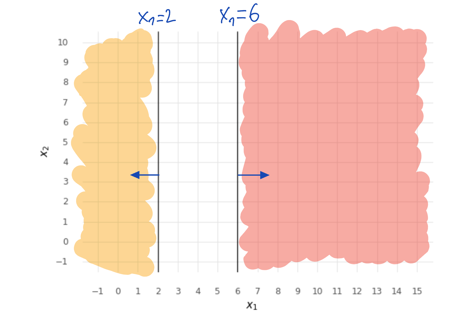
Infeasible models are the ones for which there is no feasible solution that would satisfy all the constraints. An example of an infeasible model is the following.

There is no value of 𝑥₁ which would satisfy both 𝑥₁ ≥ 6 and 𝑥₁ ≤ 2, so the intersection of the feasible half-spaces of these constraints is an empty set.
Optimisation outcome: unbounded objective
This one is a little bit weird, but unfortunately, it may occur. Usually in practise, it is a sign of an ill-defined model, e.g., when an essential constraint is not included in a model.
Unbounded objective means that for every feasible solution, we can find another feasible solution having a smaller objective value. In other words, the optimal objective value converges to negative infinity. Here is a model with an unbounded objective.

The feasible solution space is so unconstrained, that we increase 𝑥₂ to any value we want and in turn the objective will decrease.
Wrap-up
Right now, you should be able to solve any MILP model with two integer variables using just pen, paper and a ruler! Of course, the actual computer algorithms for solving MILPs are more complicated, but the visual understanding of the solution space will come handy when we study the algorithms in some future post.
All images unless otherwise noted are by the author.