


文章目录
Neural Network Representation
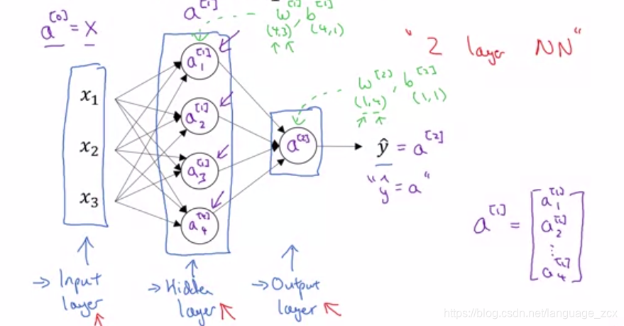
Like logistic regression architecture, you can from a Neural Network just by stacking a lot of little sigmoid units. As shown in the figure below:
Compute a Neural Network’s Output
Firstly, We set:
W [ 1 ] = [ ⋯ w 1 [ 1 ] ⋯ ⋯ w 2 [ 1 ] ⋯ ⋯ w 3 [ 1 ] ⋯ ] W^{[1]}= \begin{bmatrix} \cdots & w_{1}^{[1]} & \cdots \\ \cdots & w_{2}^{[1]} & \cdots \\ \cdots & w_{3}^{[1]} & \cdots \\ \end{bmatrix} W[1]=⎣⎢⎡⋯⋯⋯w1[1]w2[1]w3[1]⋯⋯⋯⎦⎥⎤
b [ 1 ] = [ ⋯ b 1 [ 1 ] ⋯ ⋯ b 2 [ 1 ] ⋯ ⋯ b 3 [ 1 ] ⋯ ] b^{[1]} = \begin{bmatrix} \cdots & b_{1}^{[1]} & \cdots \\ \cdots & b_{2}^{[1]} & \cdots \\ \cdots & b_{3}^{[1]} & \cdots \\ \end{bmatrix} b[1]=⎣⎢⎡⋯⋯⋯b1[1]b2[1]b3[1]⋯⋯⋯⎦⎥⎤
X = A [ 0 ] = [ ⋮ ⋮ ⋮ a [ 0 ] ( 1 ) a [ 0 ] ( 2 ) a [ 0 ] ( 3 ) ⋮ ⋮ ⋮ ] X = A^{[0]} = \begin{bmatrix} \vdots & \vdots & \vdots \\ a^{[0](1)} & a^{[0](2)} & a^{[0](3)} \\ \vdots & \vdots & \vdots \end{bmatrix} X=A[0]=⎣⎢⎢⎡⋮a[0](1)⋮⋮a[0](2)⋮⋮a[0](3)⋮⎦⎥⎥⎤
- The horizontally the matrix A/Z goes over different training examples
- The vertically the different indices in the maxtrix A/Z goes over differect hidden units of one layer
Z [ 1 ] = W [ 1 ] X + b [ 1 ] Z^{[1]} = W^{[1]}X + b^{[1]} Z[1]=W[1]X+b[1]
A [ 1 ] = g [ 1 ] ( Z [ 1 ] ) A^{[1]} = g^{[1]}(Z^{[1]}) A[1]=g[1](Z[1])
Z [ 2 ] = W [ 2 ] A [ 1 ] + b [ 2 ] Z^{[2]} = W^{[2]}A^{[1]} + b^{[2]} Z[2]=W[2]A[1]+b[2]
A [ 2 ] = g [ 2 ] ( Z [ 2 ] ) A^{[2]} = g^{[2]}(Z^{[2]}) A[2]=g[2](Z[2])
Activation Function
Why do you Need Non-linear Activation Functions?
linear activation functions just make the neural network output the linear funtion of the input no matter how many layers contains. But somtimes, linear activation functions can be used to activate the output layer or compress neural network models.
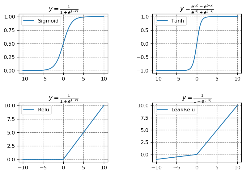
Activation Functions’ Image
import numpy as np
import matplotlib.pyplot as plt

%matplotlib inline
x = np.arange(-10, 10, 0.001)
y1 = 1 / (1 + np.exp(-x))
y2 = (np.exp(x) - np.exp(-x)) / (np.exp(x) + np.exp(-x))
y3 = np.maximum(0, x)
y4 = np.maximum(0.1*x, x)

plt.rcParams['figure.dpi'] = 120
plt.subplots_adjust(left=2, bottom=2, right=3, top=3,
wspace=0.5, hspace=0.5)

plt.subplot(221)
plt.plot(x, y1, label="Sigmoid")
plt.grid(color="gray", linestyle="--")
plt.title(r"$y=\frac{1}{1+e^{(-x)}}$")
plt.legend()

plt.subplot(222)
plt.plot(x, y2, label="Tanh")
plt.grid(color="gray", linestyle="--")
plt.title(r"$y=\frac{e^{(x)}-e^{(-x)}}{e^{(x)}+e^{(-x)}}$")
plt.legend()

plt.subplot(223)
plt.plot(x, y3, label="Relu")
plt.grid(color="gray", linestyle="--")
plt.title(r"$y=\frac{1}{1+e^{(-x)}}$")
plt.legend()

plt.subplot(224)
plt.plot(x, y4, label="LeakRelu")
plt.grid(color="gray", linestyle="--")
plt.title(r"$y=\frac{1}{1+e^{(-x)}}$")
plt.legend()
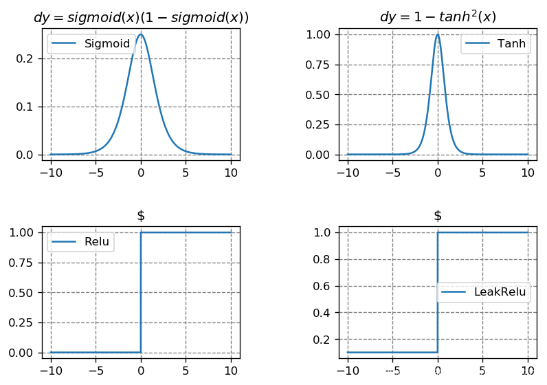
Derivatives of Activation Functions
x = np.arange(-10, 10, 0.001)
dy1 = y1* (1 - y1)
dy2 = 1 - y2 ** 2
dy3 = np.where(x>0, 1, 0)
dy4 = np.where(x>0, 1, 0.1)

plt.rcParams['figure.dpi'] = 120
plt.subplots_adjust(left=2, bottom=2, right=3 , top=3, wspace=0.5, hspace=0.5)

plt.subplot(221)
plt.plot(x, dy1, label="Sigmoid")
plt.grid(color="gray", linestyle="--")
plt.title(r"$dy=sigmoid(x)(1-sigmoid(x))$")
plt.legend()

plt.subplot(222)
plt.plot(x, dy2, label="Tanh")
plt.grid(color="gray", linestyle="--")
plt.title(r"$dy=1-tanh^{2}(x)$")
plt.legend()

plt.subplot(223)
plt.plot(x, dy3, label="Relu")
plt.grid(color="gray", linestyle="--")
plt.title(r"$")
plt.legend()

plt.subplot(224)
plt.plot(x, dy4, label="LeakRelu")
plt.grid(color="gray", linestyle="--")
plt.title(r"$")
plt.legend()
Different Choices
Recap:
If we set the 1st-convolution-layer’s parameters as W 1 , b 1 W_{1}, b_{1} W1,b1, the 2nd-convolution-layer’s parameters as W 2 , b 2 W_{2}, b_{2} W2,b2 and so on. we set a i a_{i} ai as the neural unit’s output, and the z i z_{i} zi as the output value before passing the activation function g g g.
According to the above statement, in CNN, the output of the first layer is a 1 = g ( W 1 x + b 1 ) a_{1} = g(W_{1}x + b_{1}) a1=g(W1x+b1), the output of the second layer is a 2 = g ( W 2 g ( W 1 x + b 1 ) + b 2 ) a_{2} = g(W_{2}g(W_{1}x + b_{1})+b_{2}) a2=g(W2g(W1x+b1)+b2), and the output of the third layer is a 3 = g ( W 3 g ( W 2 g ( W 1 x + b 1 ) + b 2 ) + b 3 ) a_{3} = g(W_{3}g(W_{2}g(W_{1}x + b_{1})+b_{2}) + b_{3}) a3=g(W3g(W2g(W1x+b1)+b2)+b3).
Set the final loss as L L L, let’s try to start with the third layer and use the BP algorithm to derive the bias of the loss on the parameters W 1 W_{1} W1 to see what happens.
Just for simplicity, I’m going to skip over the derivation, and the result is:
α
L
α
W
1
=
α
L
α
a
3
α
a
3
α
z
3
W
3
α
a
2
α
z
2
W
2
α
a
1
α
z
1
α
z
1
W
1
\frac{\alpha L}{\alpha W_{1}} =\frac{\alpha L}{\alpha a_{3}} \frac{\alpha a_{3}}{\alpha z_{3}}W_{3} \frac{\alpha a_{2}}{\alpha z_{2}}W_{2} \frac{\alpha a_{1}}{\alpha z_{1}} \frac{\alpha z_{1}}{W_{1}}
αW1αL=αa3αLαz3αa3W3αz2αa2W2αz1αa1W1αz1
The derivative α a 3 α z 3 \frac{\alpha a_{3}}{\alpha z_{3}} αz3αa3, α a 2 α z 2 \frac{\alpha a_{2}}{\alpha z_{2}} αz2αa2 and α a 1 α z 1 \frac{\alpha a_{1}}{\alpha z_{1}} αz1αa1 are always the chief culprit of the problem about gradient vanishing.
so choose a proper activation function is important:
-
Sigmoid – rarely use except in the output layer of a two-classes classification problem, because the output value between [0,1]
-
Tanh – The tanh activation usually works better than sigmoid activation function for hidden units because the mean of its output is closer to zero, and so it centers the data better for the next layer
-
Relu – almost used
-
LeakRelu – better than Relu
TODO:: (Improve later)
Backpropagation of Neural Network
[外链图片转存失败(img-bLCOVzbl-1565522831176)(attachment:Screenshot%20from%202019-08-02%2020-52-40.png)]
we can get the derivative below:
| single example | m examples |
|---|---|
| d z [ 2 ] = a [ 2 ] − y dz^{[2]} = a^{[2]} - y dz[2]=a[2]−y | d z [ 2 ] = a [ 2 ] − y dz^{[2]} = a^{[2]} - y dz[2]=a[2]−y |
| d W [ 2 ] = d z [ 2 ] a [ 1 ] T dW^{[2]} = dz^{[2]}a^{[1]T} dW[2]=dz[2]a[1]T | d W [ 2 ] = 1 m ( d z [ 2 ] a [ 1 ] T ) dW^{[2]} = \frac{1}{m}(dz^{[2]}a^{[1]T}) dW[2]=m1(dz[2]a[1]T) |
| d b [ 2 ] = d z [ 2 ] db^{[2]} = dz^{[2]} db[2]=dz[2] | d b [ 2 ] = 1 m n p . s u m ( d z [ 2 ] , a x i s = 1 , k e e p d i m s = T r u e ) db^{[2]} = \frac{1}{m}np.sum(dz^{[2]}, axis=1, keepdims=True) db[2]=m1np.sum(dz[2],axis=1,keepdims=True) |
| d a [ 1 ] = W [ 2 ] T d z [ 2 ] da^{[1]} = W^{[2]T}dz^{[2]} da[1]=W[2]Tdz[2] | d a [ 1 ] = W [ 2 ] T d z [ 2 ] da^{[1]} = W^{[2]T}dz^{[2]} da[1]=W[2]Tdz[2] |
| d z [ 1 ] = W [ 2 ] T d z [ 2 ] ∗ g ′ [ 1 ] ( z [ 1 ] ) dz^{[1]} = W^{[2]T}dz^{[2]} * g^{'[1]}(z^{[1]}) dz[1]=W[2]Tdz[2]∗g′[1](z[1]) | d z [ 1 ] = W [ 2 ] T d z [ 2 ] ∗ g ′ [ 1 ] ( z [ 1 ] ) dz^{[1]} = W^{[2]T}dz^{[2]} * g^{'[1]}(z^{[1]}) dz[1]=W[2]Tdz[2]∗g′[1](z[1]) |
| d W [ 1 ] = d z [ 1 ] a [ 0 ] T dW^{[1]} = dz^{[1]}a^{[0]T} dW[1]=dz[1]a[0]T | d W [ 1 ] = 1 m ( d z [ 1 ] a [ 0 ] T ) dW^{[1]} = \frac{1}{m}(dz^{[1]}a^{[0]T}) dW[1]=m1(dz[1]a[0]T) |
| d b [ 2 ] = d z [ 1 ] db^{[2]} = dz^{[1]} db[2]=dz[1] | d b [ 2 ] = 1 m n p . s u m ( d z [ 1 ] , a x i s = 1 , k e e p d i m s = T r u e ) db^{[2]} = \frac{1}{m}np.sum(dz^{[1]}, axis=1, keepdims=True) db[2]=m1np.sum(dz[1],axis=1,keepdims=True) |
Random Initialization
Reminder: The general methodology to build a Neural Network is to:
1. Define the neural network structure ( # of input units, # of hidden units, etc).
2. Initialize the model’s parameters
3. Loop:
- Implement forward propagation
- Compute loss
- Implement backward propagation to get the gradients
- Update parameters (gradient descent)
Why we need to initialize parameters randomly?
If we set W [ 1 ] W^{[1]} W[1] as np.zeros(( n [ 1 ] n^{[1]} n[1], n [ 0 ] n^{[0]} n[0])), then a 1 [ 1 ] a^{[1]}_{1} a1[1] will be equal to a 2 [ 1 ] a^{[1]}_{2} a2[1] and d z 1 [ 1 ] dz^{[1]}_{1} dz1[1] will also be equal to d z 2 [ 1 ] dz^{[1]}_{2} dz2[1] in the backpropagation. So even after multiple iterations of gradient descent each neuron in the layer will be computing the same thing as other neurons. It turns out that the hidden units in same layer are completely identical although you update the parameters many times.
To avoid the problem above, we shoud initialize the parameters randomly. So we can set:
W
[
1
]
=
n
p
.
r
a
n
d
o
m
.
r
a
n
d
n
(
n
[
1
]
,
n
[
0
]
)
W^{[1]} = np.random.randn(n^{[1]}, n^{[0]})
W[1]=np.random.randn(n[1],n[0])
b [ 1 ] = n p . z e r o s ( ( n [ 1 ] , n [ 0 ] ) ) b^{[1]} = np.zeros((n^{[1]}, n^{[0]})) b[1]=np.zeros((n[1],n[0]))
We usually prefer to initialize the weights to very small random values so that we can get a big slope and a faster learning speed when we use sigmoid or tanh activation funtion. so:
W
[
1
]
=
n
p
.
r
a
n
d
o
m
.
r
a
n
d
n
(
n
[
1
]
,
n
[
0
]
)
∗
0.01
W^{[1]} = np.random.randn(n^{[1]}, n^{[0]}) * 0.01
W[1]=np.random.randn(n[1],n[0])∗0.01

 97
97


 扫一扫
扫一扫


 被折叠的 条评论
为什么被折叠?
被折叠的 条评论
为什么被折叠?
 到【灌水乐园】发言


