PyTorch计算机视觉实战指南

原创已于 2025-11-10 10:05:44 修改 · 959 阅读

10 ·

本内容遵循CC 4.0 BY-SA版权协议

GEO检测

收录于

技术类

于 2025-11-10 09:15:00 首次发布

计算机视觉是深度学习中最具应用价值的领域之一，而PyTorch作为当前最流行的深度学习框架，以其简洁的API和动态计算图特性受到了广大研究者和开发者的青睐。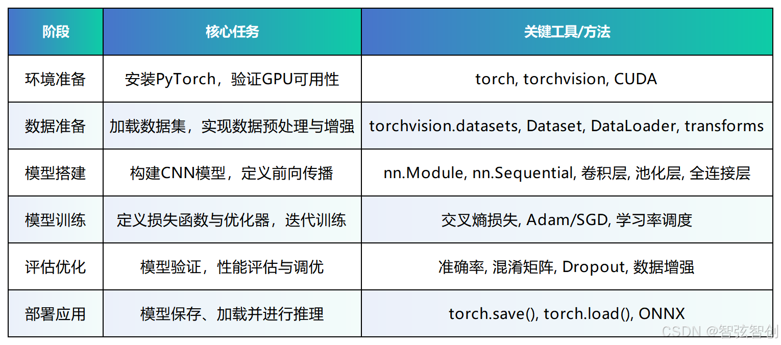

本文将带你完整走一遍使用PyTorch搭建计算机视觉模型的流程，从环境准备到模型部署，为你提供实用的代码示例和关键技术要点。

一、环境配置与验证

在开始之前，我们需要确保正确安装和配置了PyTorch环境。

1.1 安装PyTorch

访问[PyTorch官网](https://pytorch.org/)获取适合你系统的安装命令。例如，对于CUDA 11.x的用户：

pip install torch torchvision torchaudio --extra-index-url https://download.pytorch.org/whl/cu113

1.2 验证GPU可用性

安装完成后，通过以下代码验证环境配置：

import torch

print(f"PyTorch版本: {torch.__version__}")
print(f"CUDA是否可用: {torch.cuda.is_available()}")
if torch.cuda.is_available():
    print(f"CUDA版本: {torch.version.cuda}")
    print(f"GPU设备: {torch.cuda.get_device_name(0)}")

二、数据准备与预处理

高质量的数据处理是模型成功的基础。PyTorch提供了丰富的数据处理工具。

2.1 数据加载与增强

import torch
from torchvision import transforms, datasets

# 定义数据预处理流程
data_transform = transforms.Compose([
    transforms.Resize((64, 64)),           # 调整图像尺寸
    transforms.RandomHorizontalFlip(0.5),  # 随机水平翻转
    transforms.RandomRotation(10),         # 随机旋转
    transforms.ColorJitter(0.2, 0.2, 0.2), # 颜色抖动
    transforms.ToTensor(),                 # 转换为Tensor
    transforms.Normalize(                  # 标准化
        mean=[0.485, 0.456, 0.406],
        std=[0.229, 0.224, 0.225]
    )
])

# 加载CIFAR-10数据集
train_dataset = datasets.CIFAR10(
    root='./data',
    train=True,
    download=True,
    transform=data_transform
)

# 创建数据加载器
train_loader = torch.utils.data.DataLoader(
    train_dataset,
    batch_size=32,
    shuffle=True,
    num_workers=4
)

2.2 自定义数据集类

对于自己的数据集，需要继承`Dataset`类：

from torch.utils.data import Dataset
from PIL import Image
import os

class CustomDataset(Dataset):
    def __init__(self, data_dir, transform=None):
        self.data_dir = data_dir
        self.transform = transform
        self.image_paths = [os.path.join(data_dir, fname) 
                           for fname in os.listdir(data_dir) 
                           if fname.endswith(('.jpg', '.png'))]
    
    def __len__(self):
        return len(self.image_paths)
    
    def __getitem__(self, idx):
        image_path = self.image_paths[idx]
        image = Image.open(image_path).convert('RGB')
        label = 0  # 根据实际情况设置标签
        
        if self.transform:
            image = self.transform(image)
            
        return image, label

三、模型搭建：构建CNN网络

卷积神经网络是计算机视觉任务的基础架构。下面我们构建一个经典的CNN模型：

import torch.nn as nn
import torch.nn.functional as F

class SimpleCNN(nn.Module):
    def __init__(self, num_classes=10):
        super(SimpleCNN, self).__init__()
        # 第一个卷积块
        self.conv1 = nn.Conv2d(3, 32, kernel_size=3, padding=1)
        self.bn1 = nn.BatchNorm2d(32)
        
        # 第二个卷积块
        self.conv2 = nn.Conv2d(32, 64, kernel_size=3, padding=1)
        self.bn2 = nn.BatchNorm2d(64)
        
        # 第三个卷积块
        self.conv3 = nn.Conv2d(64, 128, kernel_size=3, padding=1)
        self.bn3 = nn.BatchNorm2d(128)
        
        # 池化层
        self.pool = nn.MaxPool2d(2, 2)
        
        # 全连接层
        self.fc1 = nn.Linear(128 * 8 * 8, 512)  # 假设输入为64x64，经过3次池化后为8x8
        self.dropout = nn.Dropout(0.5)
        self.fc2 = nn.Linear(512, num_classes)
        
    def forward(self, x):
        # 卷积块1
        x = self.pool(F.relu(self.bn1(self.conv1(x))))
        
        # 卷积块2
        x = self.pool(F.relu(self.bn2(self.conv2(x))))
        
        # 卷积块3
        x = self.pool(F.relu(self.bn3(self.conv3(x))))
        
        # 展平
        x = x.view(-1, 128 * 8 * 8)
        
        # 全连接层
        x = F.relu(self.fc1(x))
        x = self.dropout(x)
        x = self.fc2(x)
        
        return x

# 实例化模型
model = SimpleCNN(num_classes=10)
print(model)

关键技术点：
使用BatchNorm加速收敛并提高稳定性
添加Dropout层防止过拟合
注意特征图尺寸的变化，确保全连接层输入尺寸正确

四、模型训练与优化

4.1 定义损失函数和优化器

import torch.optim as optim

# 选择设备
device = torch.device("cuda" if torch.cuda.is_available() else "cpu")
model = model.to(device)

# 定义损失函数和优化器
criterion = nn.CrossEntropyLoss()
optimizer = optim.Adam(model.parameters(), lr=0.001, weight_decay=1e-4)

# 学习率调度器
scheduler = optim.lr_scheduler.StepLR(optimizer, step_size=10, gamma=0.1)

4.2 训练循环

def train_model(model, train_loader, criterion, optimizer, scheduler, num_epochs=20):
    model.train()
    train_losses = []
    train_accuracies = []
    
    for epoch in range(num_epochs):
        running_loss = 0.0
        correct = 0
        total = 0
        
        for i, (images, labels) in enumerate(train_loader):
            images, labels = images.to(device), labels.to(device)
            
            # 前向传播
            outputs = model(images)
            loss = criterion(outputs, labels)
            
            # 反向传播
            optimizer.zero_grad()
            loss.backward()
            optimizer.step()
            
            # 统计信息
            running_loss += loss.item()
            _, predicted = torch.max(outputs.data, 1)
            total += labels.size(0)
            correct += (predicted == labels).sum().item()
            
            if (i+1) % 100 == 0:
                print(f'Epoch [{epoch+1}/{num_epochs}], Step [{i+1}/{len(train_loader)}], '
                      f'Loss: {loss.item():.4f}')
        
        # 更新学习率
        scheduler.step()
        
        # 计算epoch统计
        epoch_loss = running_loss / len(train_loader)
        epoch_acc = 100 * correct / total
        
        train_losses.append(epoch_loss)
        train_accuracies.append(epoch_acc)
        
        print(f'Epoch [{epoch+1}/{num_epochs}], '
              f'Loss: {epoch_loss:.4f}, Accuracy: {epoch_acc:.2f}%')
    
    return train_losses, train_accuracies

# 开始训练
train_losses, train_accuracies = train_model(
    model, train_loader, criterion, optimizer, scheduler, num_epochs=20
)

五、模型评估与验证

5.1 验证集评估

def evaluate_model(model, val_loader):
    model.eval()
    correct = 0
    total = 0
    all_predictions = []
    all_labels = []
    
    with torch.no_grad():
        for images, labels in val_loader:
            images, labels = images.to(device), labels.to(device)
            outputs = model(images)
            _, predicted = torch.max(outputs.data, 1)
            total += labels.size(0)
            correct += (predicted == labels).sum().item()
            
            all_predictions.extend(predicted.cpu().numpy())
            all_labels.extend(labels.cpu().numpy())
    
    accuracy = 100 * correct / total
    print(f'Validation Accuracy: {accuracy:.2f}%')
    
    return all_predictions, all_labels, accuracy

# 假设我们有验证集 val_loader
# predictions, true_labels, val_accuracy = evaluate_model(model, val_loader)

5.2 可视化训练过程

import matplotlib.pyplot as plt

def plot_training_history(train_losses, train_accuracies):
    fig, (ax1, ax2) = plt.subplots(1, 2, figsize=(12, 4))
    
    # 绘制损失曲线
    ax1.plot(train_losses)
    ax1.set_title('Training Loss')
    ax1.set_xlabel('Epoch')
    ax1.set_ylabel('Loss')
    
    # 绘制准确率曲线
    ax2.plot(train_accuracies)
    ax2.set_title('Training Accuracy')
    ax2.set_xlabel('Epoch')
    ax2.set_ylabel('Accuracy (%)')
    
    plt.tight_layout()
    plt.show()

plot_training_history(train_losses, train_accuracies)

六、模型部署与推理

6.1 保存和加载模型

# 保存完整模型
torch.save(model, 'complete_model.pth')

# 保存模型状态字典（推荐）
torch.save(model.state_dict(), 'model_weights.pth')

# 加载模型
# 方法1：加载完整模型
model = torch.load('complete_model.pth')

# 方法2：加载状态字典（需要先创建模型结构）
model = SimpleCNN(num_classes=10)
model.load_state_dict(torch.load('model_weights.pth'))
model.eval()  # 设置为评估模式

6.2 单张图像预测

from PIL import Image

def predict_single_image(image_path, model, transform, class_names, device):
    # 加载和预处理图像
    image = Image.open(image_path).convert('RGB')
    image_tensor = transform(image).unsqueeze(0)  # 增加批次维度
    image_tensor = image_tensor.to(device)
    
    # 预测
    with torch.no_grad():
        outputs = model(image_tensor)
        probabilities = F.softmax(outputs, dim=1)
        confidence, predicted = torch.max(probabilities, 1)
    
    predicted_class = class_names[predicted.item()]
    confidence_score = confidence.item()
    
    return predicted_class, confidence_score

# 使用示例
# class_names = ['airplane', 'automobile', 'bird', 'cat', 'deer', 
#                'dog', 'frog', 'horse', 'ship', 'truck']  # CIFAR-10类别
# predicted_class, confidence = predict_single_image(
#     'test_image.jpg', model, data_transform, class_names, device
# )
# print(f'Predicted: {predicted_class}, Confidence: {confidence:.4f}')

七、进阶技巧与优化

7.1 使用预训练模型（迁移学习）

import torchvision.models as models

# 加载预训练的ResNet模型
def create_pretrained_model(num_classes=10):
    model = models.resnet18(pretrained=True)
    
    # 冻结所有层（可选）
    # for param in model.parameters():
    #     param.requires_grad = False
    
    # 替换最后的全连接层
    num_features = model.fc.in_features
    model.fc = nn.Sequential(
        nn.Dropout(0.5),
        nn.Linear(num_features, num_classes)
    )
    
    return model

pretrained_model = create_pretrained_model(num_classes=10)
pretrained_model = pretrained_model.to(device)

7.2 模型轻量化技术

# 模型量化示例（推理时减少内存占用和加速）
model_quantized = torch.quantization.quantize_dynamic(
    model, {nn.Linear}, dtype=torch.qint8
)

# 使用TorchScript优化
traced_script_module = torch.jit.trace(model, torch.rand(1, 3, 64, 64).to(device))
traced_script_module.save("traced_model.pt")

八、完整项目结构建议

一个良好的PyTorch项目应该包含以下结构：

cv_project/
│
├── data/
│   ├── raw/           # 原始数据
│   ├── processed/     # 处理后的数据
│   └── datasets.py    # 自定义数据集类
│
├── models/
│   ├── __init__.py
│   ├── base_model.py  # 基础模型类
│   ├── cnn.py         # CNN模型定义
│   └── utils.py       # 模型工具函数
│
├── training/
│   ├── train.py       # 训练脚本
│   ├── evaluator.py   # 评估脚本
│   └── config.py      # 训练配置
│
├── utils/
│   ├── visualization.py  # 可视化工具
│   └── helpers.py     # 辅助函数
│
├── notebooks/         # Jupyter notebooks
├── requirements.txt   # 依赖列表
└── README.md         # 项目说明