寒假学习Day 12:Python 绘图

寒假学习Day 12:Python 绘图

参考文章：
https://blog.csdn.net/rosefun96/article/details/84259816?ops_request_misc=&request_id=&biz_id=102&utm_term=Python%25E7%25BB%2598%25E5%259B%25BE&utm_medium=distribute.pc_search_result.none-task-blog-2_allsobaiduweb~default-5-84259816.nonecase

用到的库

import matplotlib.pyplot as plt
import numpy as np
from mpl_toolkits.mplot3d import Axes3D
import cv2
 

柱状图

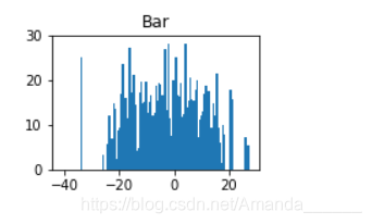
n=1024
X=np.random.normal(0,10,n)#正态分布（均值，标准差，shape）
Y=np.random.normal(0,10,n)
 
fig=plt.figure
plt.subplot(221)#设置位置
plt.title("Bar")
plt.bar(X,Y)
plt.xlim()
plt.ylim(0,30)
plt.show()

plt.subplot(221) # 第一行的左图
plt.subplot(222) # 第一行的右图
plt.subplot(212) # 第二整行
plt.show()

其中各个参数也可以用逗号,分隔开。第一个参数代表子图的行数；第二个参数代表该行图像的列数； 第三个参数代表每行的第几个图像。

折线图

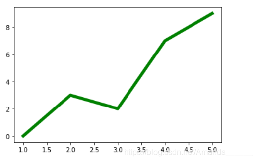
x = [1,2,3,4,5]
y = [0,3,2,7,9]
 
plt.figure()
plt.plot(x, y,'g-', lw =5)
plt.show()

热力图

方法一

import numpy
import matplotlib.pyplot as plt
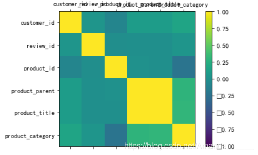
correlations = data.corr()  #计算变量之间的相关系数矩阵
# plot correlation matrix
fig = plt.figure() #调用figure创建一个绘图对象
ax = fig.add_subplot(111)
cax = ax.matshow(correlations, vmin=-1, vmax=1)  #绘制热力图，从-1到1
fig.colorbar(cax)  #将matshow生成热力图设置为颜色渐变条
#ticks = np.arange(10)
# ax.set_xticks(ticks)  #生成刻度
# ax.set_yticks(ticks)
names = data.columns.tolist()
ax.set_xticklabels(names) #生成x轴标签
ax.set_yticklabels(names)
plt.show()

方法二

import pandas as pd
import numpy as np
import matplotlib.pyplot as plt
import seaborn as sns
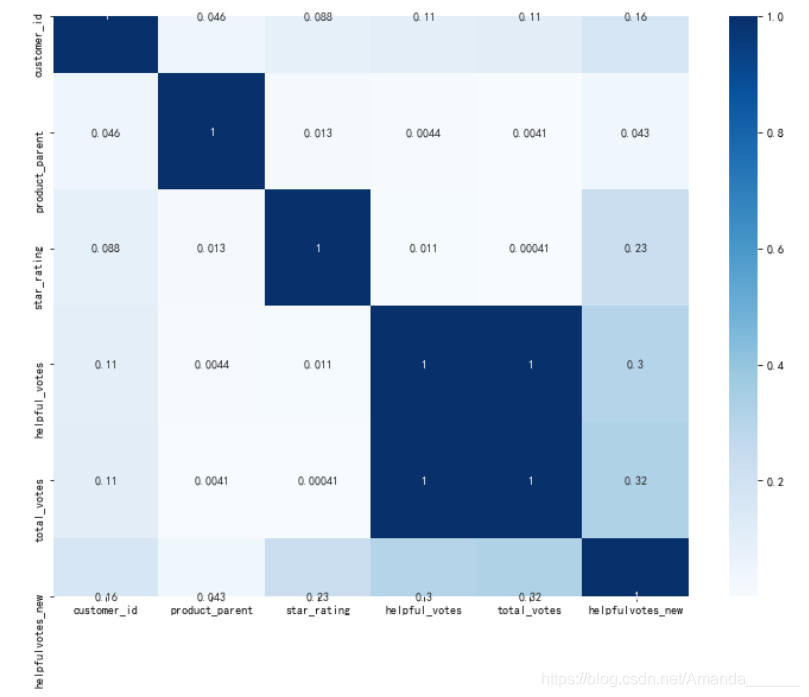
data_corr=dataset.corr().abs()

plt.figure(figsize=(12,9))
print(" the correlation between features :")
sns.heatmap(data_corr,annot=True,cmap='Blues')

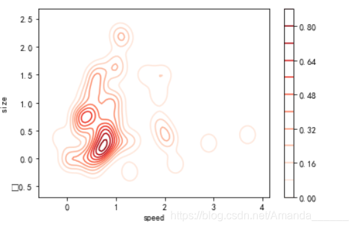
二维密度图

# Importing libs
import seaborn as sns
import matplotlib.pyplot as plt
from scipy.stats import skewnorm

# Create the data
speed = skewnorm.rvs(4, size=50) 
size = skewnorm.rvs(4, size=50)

# Create and shor the 2D Density plot
ax = sns.kdeplot(speed, size, cmap="Reds", shade=False, bw=.15, cbar=True)
ax.set(xlabel='speed', ylabel='size')
plt.show()

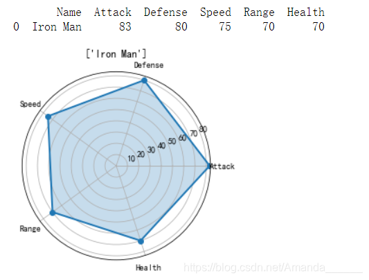
蜘蛛网图

# Import libs
import pandas as pd
import seaborn as sns
import numpy as np
import matplotlib.pyplot as plt

# Get the data
df=pd.DataFrame(index = [0], columns = ['Name', 'Attack', 'Defense', 'Speed',
                'Range', 'Health'], data = [['Iron Man',83, 80, 75, 70, 70]])
print(df)

"""
   #             Name  Attack  Defense  Speed  Range  Health
0  1         Iron Man      83       80     75     70      70
1  2  Captain America      60       62     63     80      80
2  3             Thor      80       82     83    100     100
3  3             Hulk      80      100     67     44      92
4  4      Black Widow      52       43     60     50      65
5  5          Hawkeye      58       64     58     80      65

"""

# Get the data for Iron Man
labels=np.array(["Attack","Defense","Speed","Range","Health"])
stats=df.loc[0,labels].values

# Make some calculations for the plot
angles=np.linspace(0, 2*np.pi, len(labels), endpoint=False)
stats=np.concatenate((stats,[stats[0]]))
angles=np.concatenate((angles,[angles[0]]))

# Plot stuff
fig = plt.figure()
ax = fig.add_subplot(111, polar=True)
ax.plot(angles, stats, 'o-', linewidth=2)
ax.fill(angles, stats, alpha=0.25)
ax.set_thetagrids(angles * 180/np.pi, labels)
ax.set_title([df.loc[0,"Name"]])
ax.grid(True)

plt.show()